Challenges in Well Testing Data from
Multi-layered Reservoirs and Improving Nonlinear
Regression: A Gas filed case
Sh. Soleimani 1,*, A. Hashemi 1, R. Kharrat 1
1 Department of Petroleum Engineering, Science and Research branch, Islamic Azad
University, Tehran, Iran.
ARTICLE INFO ABSTRACT
Article history:
Received: June 17, 2017 Accepted: December 19, 2017
Keywords:
Numerical Simulation
Automated Type-curve Matching Minimizing the Analyzer Error Multilayer Gas Reservoirs
* Corresponding author;
E-mail: [email protected]
1. Introduction
The interpretation of multi-layer reservoir is almost unsuccessful without an awareness of each layer features. In a multi-layer reservoir, pressure and pressure derivative plot in a model do not show the features of each layer since the down hole pressure depends on the whole system and layers [1]. In a multi-layer reservoir, each multi-layer has different production rates at different times [2], therefore, using the total flow rates in the surface to predict each layer is wrong. In this regard, in addition to pressure data, measuring flow rate of each layer is required to calculate features and parameters [3, 4]. The analysis using matching of measured data in the semi-logarithmic and logarithmic plots requires the properties of flow rate and pressure [5]. The major problem for layered systems is still estimating Individual layer permeability and skin factors from conventional well tests. The conventional drawdown and buildup tests usually reveal only the behavior of the total system. Furthermore, the behavior of a multilayer formation may not be distinguished from the behavior of a single layer formation.
The principal objective of this study was to investigate methods of improving the type curve matching procedure automatically for multilayer gas reservoirs instead of trying to analyze the individual layer production histories and pressure data. In this respect, the present work proposes estimation of individual layer properties by simultaneously type curve matching the total well pressure change and its derivative. In addition to field studies and practical jobs of multi-layered reservoirs well testing, there is another method using the computer well test analyzer and reservoir simulation software (Eclipse 100)1, which is explained in the next sections.
Software companies improve their relations and formulas with the coefficients they earn in laboratories. They try to get results close to reality, but these conditions are usually obtained in conditions related to fluid and rock information of reservoir of their own domain. Actually they make the formulas homemade. As a same input may result in different at two applications, it is possible to make more errors with our oil and gas reservoir information. So, two ways are available: measure the error rate using design synthetic models of reservoir or using homemade relationships.
2. Literature review
Various studies have been conducted in the context of estimating parameters of each layer with some of them providing highly accurate results. With respect to layered reservoirs, as one type of reservoir heterogeneity considered in this study, the most extensive study in this area is by Tariq [6] in 1977 in which type curves were generated for a bounded multilayered system without cross-flow between the layers. Jahns [7] used a combination of reservoir simulation and regression analysis to describe a two-dimensional reservoir from data of interference tests. He divided the reservoir into a number of homogeneous blocks whose transmissibility (kh/µ) and storativity (Øct h) were estimated to satisfy the least-square criterion. From 1980s to 1990s, many researchers interpreted well testing data by the analysis of measured wellbore pressure and
stratified flow rate. Lolon and Archer [8] introduced a semi-analytical method for downhole pressure for multi-layer reservoirs without the flow rate between layers. They also obtained a relation to calculate total pressure and flow rate of each layer. With the aid of multilayer testing techniques, the expression of pressure solution was established through the relationship between wellbore pressure and stratified flow rate of multilayered reservoir [9, 10]. In recent years, numerical methods have been employed to study well testing problems of multilayered reservoir with the aid of computer technology rapid development [11].
The first use of computer-aided well test analysis dates back to the 1960s. Jacquard and Jain (1965) divided a single layered reservoir into a number of homogeneous blocks of constant reservoir properties to interpret interference tests, and used regression analysis techniques to estimate the permeabilities of the blocks. Barua et al. (1988) considered practical problems that could be raised in the application of automated well test analysis due to poor initial estimates or inherently ill-defined parameters. Their major objective was to find an alternative regression algorithm when the popular Gauss-Marquardt method failed.
3. Methodology
To analyze the well, it is needed at least to have the pressure data against time. Also, the production rate of each layer and its use in the analytical analysis significantly decreases the error. Therefore, by using the known keywords of the final data file, the numerical results of downhole pressure and the overall well production as well as production of each layer against time as the numerical output were obtained. Different scenarios are permeable. Skin contrasts between the layers were designed, and the simulation responses were exported to an analytical well test package. In addition, the tests were analyzed as actual tests, and finally to gain the least final error of the results, a practical interpretation methodology was achieved.
3.1. Numerical simulation (synthetic example)
Table 1. The overall information of simulated reservoir
Property Layer 1 Layer 2 Shale
Porosity (%) 13 13 0
Perm Z (md) 0 0 0
Perm R (md) 4 100 0
Perm ϴ (md) 4 100 0
Rock Comp(psi-1) 1.2E-5 1.2E-5 1.2E-5
Skin 0 0 0
Thickness (ft) 125 125 10
Depth (ft) 7500 7635 7625
Table 2. The production rate and well characteristics
Property Info
Gas rate (Mscf/Day) 20000 Reservoir phase Dry Gas Number of wells 1
3.1.1. Applied conditions to the reservoir simulation model
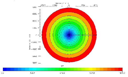
To better simulate and decrease the calculation errors, specific conditions were applied. In the reservoir model, logarithmic time steps were used, which in fact, included pressure record and calculation steps. In this respect, time steps and very few time steps were initially designated to observe the reservoir primary effect, and the reservoir radius changes were introduced as logarithmic as follows:
Figure 1. The logarithmic radius changes
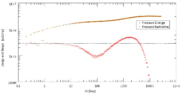
3.1.2. The sub-layer increase and its effect on the reservoir numerical simulation
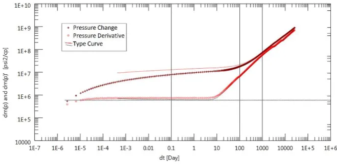
Figure 2. Log-Log plot when number of sub-layers is not defined. (Layer 1 permeability 40 md & layer 2 permeability 100 md)
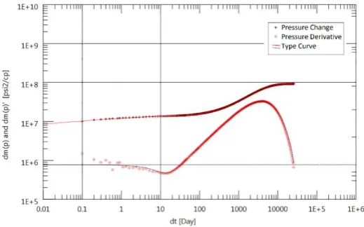
Figure 3. Log-Log plot when number of sub-layers increased to 30. (Layer 1 permeability 40 md & layer 2 permeability 100 md)
3.2. Well test analysis, analytical
Numerical output of reservoir simulation resultants was used as input data of well analyzer to obtain each layer parameters and then each layer parameters by means of type curve matching was determined. In the case of incomplete matches with the type curves, we changed some of the model parameters until the best plot was obtained, indicating the real state of reservoir. Saphir1 software from Ecrin family was used. To analyze well and obtain true resultant, first the general information, including well radius, porosity, fluid type and fluids flow pattern, total thickness of layers, properties of fluid used in the simulation must be entered accurately, and reservoir type must inevitably be selected multi-layer, otherwise, the analyzer would designate the reservoir as single layer (In the “main option” window). After that the analyzer plots the production history, by selecting the pressure build-up zone to plot the pressure derivative diagram, the analysis
began. The analyzer will surmise initial guess which caused large error and it did not good match with the all points (Figure 4). Then we reduced the error by applying the modifications to the analyzer and changing the reservoir model.
Figure 4. Initial match by Saphir (buildup)
3.3. Regression points modification
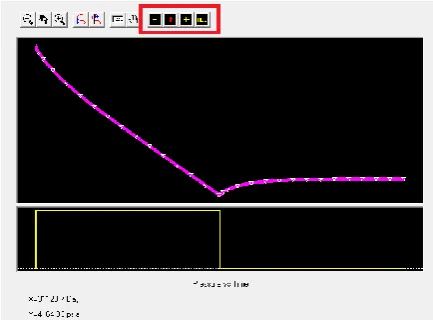
The points used to compare the result of numerical analysis and type curve were selected by software as default, and we can apply changes, including adding points, deleting points and selecting all points in the cases of Log-Log plot and simulation. Simulation for production history and pressure was applied as the type curve matching, and in the case of Log-Log, these points are selected in respect to the pressure derivative plot. As we can see in following, these points are selective and changeable:
Figure 6. Regression points window in the analyzer in the case of Log-Log
The wrong selection of these points in the parts like “shut in” may change the whole results. This method is useful in the case of resultant information from the real well test in which large scattering in its pressure derivative plot is observed.
3.4. Modification of each layer efficiency coefficient
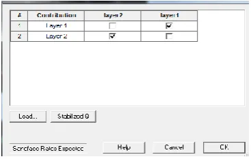
Adding each layer production for multi-layer reservoir separately and modifying each layer efficiency coefficient improve the results [12]. A function (each layer efficiency coefficient) has been defined for each layer effect in the software, which is almost the ratio of “Kh” of layers. Before improving, we add each layer production rate to the analyzer and activate it as the following figure, then in the “improve” window, we inevitably activate the layer rate:
Figure 7. Adding each layer production rate separately.
Table 3. Layer efficiency coefficient before and after modification
Initial layer efficiency coefficient Modified layer efficiency coefficient
Layer 1 0.5 0.04
Layer 2 0.5 0.96
3.5. The best initial guess
analyzer select every plot of model to determine the resultant of parameter changes.
Figure 8. Analyzer improve window
We face two choices of Log-Log and simulation (History matching), which first one is based on comparing the results with pressure derivative, and the second one is to conform production history and pattern plot pressure that one of them must provide a better result. The activation of Log-Log case choice provides accurate results relative to the simulation case, therefore, simulation case can modify the initial analyzer guess. Now, we select the simulation. Although the software is in good agreement with the results, parameters values are significantly different from the numerical simulation values, which can be used as a good initial guess:
Figure 10. The analyzer matching in the case of simulation in the buildup zone.
Then, we had proper initial guess, and had entered the production rate of the layers, and have not unfavorable points in the regression points. Thus, we improve the obtained simulation result with Log-Log choice.
Figure 11. Analyzer matching in the Log-Log state in the buildup zone (after simulation case)
Table 4. The comparison of obtained result of proposed applied method with the real values Error percentage Log-Log case results Error percentage Simulation case results Numerical simulation Property ---0.45 -- -0.45 0 S-first layer --0.000769 -- 7.11 0 S-second layer 11.25 % 3.55 20% 4.8 4 md K-first layer 4.16 % 95.84 25.36% 125.36 100 md K-second layer 6.24 % 8203.02 19.30% 9211.85
7721 ft Re-first layer 13.1 % 8732.72 6.1% 7665.15 7721 ft Re-second layer
If we selected all of the Log-Log plot points for the regression, we would definitely obtain a better result. The selection of all of the plot points is not recommended when the error is large, since with respect to the number of unknowns and points for the calculation, it is highly time-consuming to obtain result and converge, but if the error is very little, the result is obtained with more accuracy, less time and low number of steps. Therefore, we entered the regression selection part to reduce the error and point to point conformation of the pattern plot, and click the all points choice. Accordingly, as Table 5 shows, the final results from the proposed method had very little error that is acceptable:
Table 5. The final analysis result by selecting all of the regression points Analysis without proposed method (only log-log case) Proposed method analysis Property 5.4991 0 S-first layer 8.9079 0 S-second layer 6.0322 3.7215
K-first layer (md)
94.6494 95.5076
K-second layer (md)
8501.97 8203.79
Re-first layer (ft)
8442 8732
Re-second layer (ft)
4. The analysis of real field well test result
In this study, we determined the obtained well test result of SPD3-XX drilled in the South Pars field. It consisted of four layers namely K1, K2, K3 and K4 by using the above-mentioned method.
Table 6. Reservoir rock and fluid properties
properties Method or Value
Z Dranchuk
Mug Carr et al
Bg 0.0042 cf/scf
Net Pay K2 60.7 ft Net Pay K3 196.85 ft Net Pay K4 416.67 ft
Prosave K2 9.71
Prosave K3 5.92
Prosave K4 16.32
Gas saturation 100 % Well Radious 7”
Ct 2.7 E-6
4.1. The initial guess improvement with the last layer separate analysis
This well was designated as a dry gas production well with respect to negligible condensate production until the approximation of result was close by the mentioned method, and the well test was conducted in K2, K3 and K4 layers.
Table 6. The analysis result of layer K4 and its comparison with real values
Error percentage Real value Analysis Property 5.7 % -3.5 -3.30 S 2% 36.71 35.94 K (md)
First, we entered the analysis of K4 layer as the initial value for this layer, then we improved the initial guess by using the simulation analysis, which is based on regression error analysis, with respect to that there is a lot irregularity in the history and pressure derivative plot, using all of the points since regression points increases the result error. So, the points must be selected manually. Finally, the authors obtained the following result by the initial guess of K4 layer:
Table 7. Result of layers K2, K3.
Error percentage Real value Analysis Property 7.3% -0.82 -0.76 S2 11.11% 40.02 44.47 K2 (md)
4.23% -1.78 -1.8554 S3 18.41% 18.73 22.18 K3 (md)
Next, we activated the skin effect and permeability values to reduce error and changes until a new result would be obtained (Table 8):
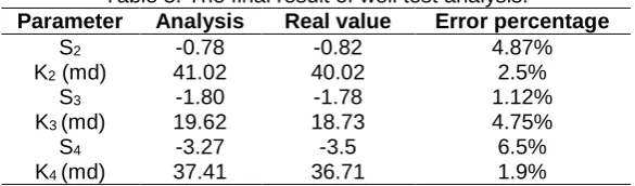
Table 8. The final result of well test analysis.
Error percentage Real value Analysis Parameter 4.87% -0.82 -0.78 S2 2.5% 40.02 41.02 K2 (md)
1.12% -1.78 -1.80 S3 4.75% 18.73 19.62 K3 (md)
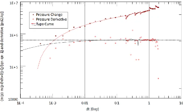
Figure 13. Default matching of analyzer on well 'SPD3' of South Pars field
Figure 14. Analyzer matching using the explained methodology on well 'SPD3' of South Pars field
5. Result and Discussion
(Log-Log) as a good initial guess in Ecrin software. The true selection of regression points can reduce the error, but when there is high irregularity in the regression points, it causes the error increase.
6. Conclusion
It is better to put the time steps as logarithmic series for the numerical simulation and the selection of radius changes as logarithmic contributes to the analysis results.
Simulation of multi-layer reservoir shows uniform results in the pressure derivative plot as the layers increase to the sub-layers.
Using each layer production rate contributes to the reduction of error. Therefore, it is necessary to modify each layer weight coefficient in Ecrin software. This value is almost equal to the Kh ratios for each layer.
The true selection of regression points can reduce the error.
To decrease the unknowns of each layer, parameters of multi-layer reservoir can find the last reservoir layer parameters separately as a single layer reservoir used in the multi-layer analysis.
References
[1] H. PARK, “well test analysis of a multilayered reservoir with formation crossflow,” 1989.
[2] H.A. Eskandari Niya M., A. Zareiforoush, “Challenges in Well Testing Data from Multi-Layered Reservoirs; a Field Case,” Int. J Sci. Emerging Tech, vol. 4, 2012.
[3] P.R. Raghavan R., A.C. Reynolds, “Well Test Analysis for Wells Producing Layered Reservoirs with Crossflow,” Soc. Pet. Eng. J., pp. 407-418, June 1985.
[4] A.J. Rosa, R.N. Horne, “Automated Type-Curve Matching in Well Test Analysis Using Laplace Space Determination of Parameter Gradients,” presented at the 58th Annual Technical Conference and Exhibition, San Francisco, CA, 1983.
[5] J.P. Spivey, “Estimating Layer Properties for Wells in Multilayer Low-Permeability Gas Reservoirs by Automatic History-Matching Production and Production Log Data,” presented at the Gas Technology Symposium, Calgary, Alberta, Canada, 2006.
[6] S.M. Tariq, “A Study of the Behavior of Layered Reservoirs with Wellbore Storage and Skin Effect,” Ph.D. Dissertation, Petroleum Engineering Department, Stanford University, 1977.
[7] H.O. Jahns, “A Rapid Method for Obtaining a Two-Dimensional Reservoir Description From Well Pressure Response Data,” Soc. Pet. Eng. J., December 1966.
[8] A. R. A. Lolon E.P., T.A. Blasingame, “New Semi-Analytical Solutions For Multilayer Reservoirs,” p. 8, 2008.
[10] S. P. C. Kuchuk F., L. Ayestaran, B. Nicholson, “Application of multilayer testing and analysis: a field case,” presented at the in Proceedings of the SPE Annual Technical Conference and Exhibition, New Orleans, La, USA, 1986.
[11] H.G. Haiyang Yu, Y. He, H. Xu, L. Li, T. Zhang, B. Xian, S. Du, Sh. Cheng, “Numerical Well Testing Interpretation Model and Applications in Crossflow Double-Layer Reservoirs by Polymer Flooding,” The Scientific World Journal, 2014.