Adapting Enhanced the Simultaneous Localization and Mapping (SLAM) Process
Based on Artificial Neural Network
Musa A Hameed Al Douri, Hussein H Owaied Faculty Information Technology
Middle East University Amman, Jordan
ABSTRACT: Different systems were implemented for environments mapping and navigation. Simultaneous Localization and Mapping process is considered an important one of them, this process allowed humans to be able to navigate and draw maps for environments where humans are not able to get through. Using several methods of preparing datasets for the landmarks of an environment, SLAM was able to navigate and build its own map of landmarks based on them. In our work, we benefitted from previous approaches design an enhanced SLAM system, which is based on Artificial Neural Network. However, by training this network on real dataset of environments, our proposed system was able to navigate an environment and build its own map accurately and without prerequisite.
Keywords: SLAM (Simultaneous Localization and Mapping), ANN (Artificial Neural Network), EKF (Extend Kalman Filter)
Received: 8 May 2013, Revised 10 June 2013, Accepted 17 June 2013
© 2013 DLINE. All rights reserved
1. Introduction
For a long time, the researchers and developers concentrated their efforts on developing intelligent machines capable of doing tasks in dangerous or remote environments. To give humans more time to devote to their leisure, or take less risk to perform dangerous tasks. The Simultaneous Localization and Mapping (SLAM) problem focuses on the possibility for a mobile robot to exist at an unknown location in an unknown environment, and the ability of this robot to build a consistent map of this environment and giving simultaneous coordinates to its location. The solution to this problem provides a great achievement in the robotics field as it provides the ability for a robot to be autonomous.
SLAM has been performed theoretically in different forms; it is also implemented in different domains, such as, indoor, outdoor and underwater environments. Probabilistic SLAM problem was first proposed at the IEEE Robotics and Automation Conference on 1986. Many researchers had been working on applying estimation-theoretic methods to environment mapping and localization problems. Few years later a new statistical method was established by Smith, Cheesman and Durrant-White [1] [2]. This statistical basis for measuring the relationships between landmarks in addition to manipulating geometric uncertainty. They showed in their work that there must be a high degree of correlation between the estimation of different landmark locations in the map, which grows with successive observations.
fusion navigation, resulted in enhancing the landmark representation of the environment, other researches based on visual methods allowed a mobile robot to move through an unknown environment taking relative observations of landmarks [4] [5]. Taking in account the high correlation between the estimates of these landmarks, due to the margin of error in the estimated vehicle location [6].
The landmarks positions in addition to the vehicle situations shape a full solution to the localization and mapping combined problem. However, a huge state vector required to be implemented scaling the number of landmarks in the map. Estimating that the mapping error would not converge and would grow without bounds. Thus, the researchers considered the complexity of the mapping problem computations only, regardless of its convergence, they focused their attention on a sequence of approximations to the solution of the localization and mapping problem. Their method considered minimizing the high correlation between the landmarks, resulted in reducing the usage of filter to a series of decupled landmark to vehicle filter [7] [8].
At the 1995, International Symposium on Robotic Research [9], SLAM problem structure and the results of the convergence was first presented. Recently, several researches and approaches were proposed on the theory of convergence, such as [10] [11]. Also on localization and mapping, such as [12] [13] [14] [15] [16] [17] [18], working on indoor, outdoor and underwater environments. The enhancements on SLAM problem developed to focus on adding many skills on robots to be autonomous, such as detecting objects in the environment, locating them and recognizing them, these features gives the robot more abilities, such as, obstacle avoidance and tasks handling. In this work, we will propose an enhanced SLAM algorithm based Artificial Neural Network (ANN), in order to enhance the robot estimations of landmarks and then the robot position on the map with high accuracy.
Beside this section, we will explain the SLAM algorithms and methods in the second section. We will explain our approach and the used algorithms in the third section. In the fourth section, we will discuss our results. Finally, we will conclude and summarize our work in the fifth section.
2. Explaining SLAM
2.1 Kalman Filter
The main idea of SLAM process is to give the ability of the robot to build a map for an environment and at the same time use this map to find its location in this environment [20] [21]. Without previous knowledge of the environment SLAM process estimates the trajectory of the environment and the landmarks, in addition to the robot continuous position on real time. It is noticed from the definition that SLAM is responsible for two main tasks; initially it is responsible for the localization of the robot. Then it is responsible for mapping the studied environment. Enhanced by Kalman filter, it was proofed by Durrant-Whyte et.al. That the mapping performance of the environment could be achieved without previous readings, and with good performance, hence the robot observations and the sensors readings are almost alike.
In figure 1 below, we considered a mobile robot supported with a sensor, moving through an environment model. The task of the
robot is to take relative readings of unknown landmarks in the environment at an instant time k. While:
xk : The state vector, defining the location of the robot.
mi : Vector for the location of the ith true landmark.
uk : Control Vector applied at time k− 1 to find the state vector xk at time k.
zik : The value of the observation taken from the robot of the location of the ith landmark at time k.
There are three parameters should be considered in the SLAM process in order to give a complete map of an environment: the mobile robot position, the landmark process model and the environment model.
2.2 Mobile Robot Position
Whatever the domain of application the robot is intended to be used, it should satisfy certain level of autonomy in localization
and navigation. Simply it should find answers to the following three solutions: “Where am I?”, “Where do I go?”, and “How to
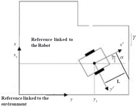
In our work, we are studying the mapping on a 2D plane. This includes all the information needed for a robot to build its map. This mapping process includes, localizing the robot itself, then determining the Cartesian coordinates for the position and angle of orientation related to the environment.
Figure 1. SLAM elements and observations
Figure 2. Formalization of the parameters for the localization process
As shows in figure 2 above, there are several parameters needed to be calculated for a robot to determine its position in the environment. Where:
Reference linked to the Robot
x xr
y yr
yr
xr
Reference linked to the environment
L
α
x′ = V cos ∅′
y′ = V sin ∅′
∅′ = v tan L γ
Which give us the nonlinear parameters of the localization function f (x, y, ∅). Then the location can be determined by:
x (k + 1) y (k + 1)
∅ (k + 1)
x (k) + ∆tV(k) cos ∅(k) y (k) + ∆tV(k) sin ∅(k)
∅(k) + ∆tV(k) tan γ (k) L
⎣
⎡
⎤
⎦
=⎣
⎡
⎤
⎦
+ w (k)Where, w is the noise at time k.
Several techniques have been developed to ensure accurate knowledge of the robot position in the environment. They are classified into two main categories: Location relative, and location absolute. In the first one, the position is calculated by incrementing the previous position of the variation measured by proprioceptive sensors; this category contains two main methods: Odometry and initial location. The second category the position calculated by the position relative to fixed pins through exteroceptive sensors, this also requires knowledge of the environment.
Different techniques can be distinguished by the nature of the landmarks used or the method of calculation. Depending on the nature of the landmarks used, the most known approaches are the Magnetic Compass localization and Active Beacons localization. The landmark navigation and the localization based on the model are distinguished according to the computational techniques used among other methods based on trilateration (or multilateration), methods based on triangulation.
3. Landmark Process Model
As it is mentioned earlier, there are several types of landmarks, with different measurement methods.
3.1 Magnetic Compass
Magnetic compass is used to determine an absolute direction by measuring the horizontal component of the earth magnetic field, in this type; the landmark is linked with the land. The main drawback of Magnetic compass is the fact that this field is altered near the power lines or large metal structures.
3.2 Active Beacons
Tags are placed at known locations in the environment. They are easily detected by the robot and with a low computational cost. To locate the landmarks, the mobile robot is equipped with a transmitter and receiver or vice versa tags. The advantage of such a system is the high sampling rate. The disadvantages are the difficulty of placing the tags on the accurate positions, in addition to the installation and maintenance costs. The calculation of the position and the orientation is based on trilateration or triangulation.
3.3 Landmarks Measurement Using Two Points
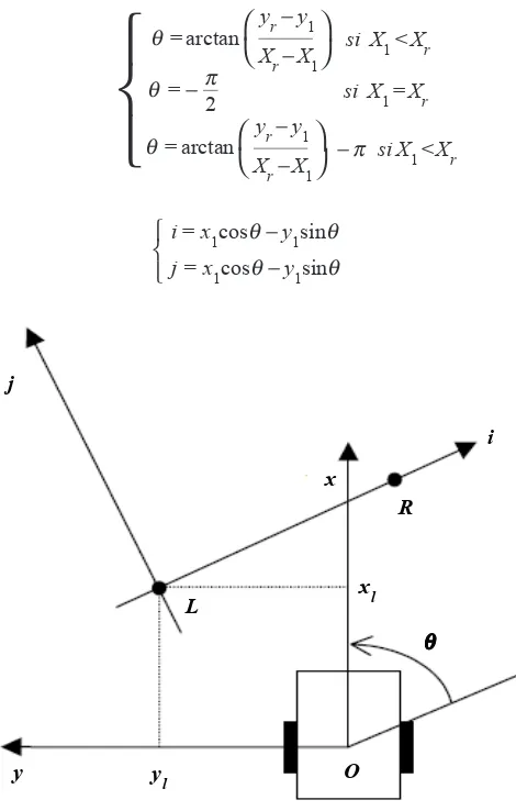
A camera and a laser plane are used. A cut of the environment is done by laser. Two points R(xr , yr ) and R(xl , yl) in the frame of the robot Rr, are extracted from this cup. As shown in figure 3 below, a landmark Rij is defined by these two points: the transition matrix of Rij in Rr is:
ijTr =
Orientation and position are then obtained as follows:
θ = arctan yr − y1
Xr − X1 si X1 <Xr
⎝
⎛
⎠
⎞
θ = − π2 si X1 =Xr
θ = arctan yr − y1
Xr − X1 − π si X1 <Xr
⎝
⎛
⎠
⎞
⎨
⎩
⎧
And
i = x1cosθ− y1sinθ
j=x1cosθ− y1sinθ ⎨
⎩ ⎧
Figure 3. Localization through two points
3.4 Environment Model
The first mobile robots were called Automated Guided Vehicles (AGVs). These are systems designed almost exclusively for industrial repetitive tasks such as transporting loads along a single path environment. This task was performed with reflective stripes, a white line on the ground, or through electromagnetic buried cables. Since mobile robots are increasingly being developed for indoor applications, such as disabled person assistance in an apartment, or guiding visitors in a museum. These applications share a common environment that can be described as semi-structured environment. While it is possible to equip an industrial environment by tags or artificial landmarks, this is hardly feasible in a home or office environment.
The approach of location and type of the environment model are strongly linked. Whatever approach is used, the location in the context of an internal environment can be divided into two problems which will be designated by incremental localization and global localization. Incremental localization implies the existence at any time even a rough estimate of the position and orientation of the robot, which facilitates the matching task with the model. In some cases, there are no estimates available. The localization problem is more complex because of the symmetries and ambiguities.
4. Proposed Algorithm
In the previous section, we studied the SLAM process, methods and algorithms, in which we developed our design of our proposed idea. In this section, we will explain our proposed algorithm, and new approach of using Artificial Neural Network
j
x
R
i
L
y yl O
xl
(ANN), to enhance the mapping process.
After studying the SLAM algorithms and methods, we propose an enhanced SLAM algorithm based on Artificial Neural Network. In our algorithm, we used the equations of the SLAM landmark equations to train our neural network; we also used a landmark dataset from Drexel Autonomous System Lab datasets, which where scanned using SICK scanner [23].
Together with the landmark equations, we trained the neural network to obtain enhanced results of SLAM landmarks, and then enhanced robot maps. In order to obtain this result we need to model this process initially. In our algorithm, we supposed a known dataset of landmarks, GPS coordinates of our map, due to the egg, and chicken problem in SLAM, a dataset of landmarks is needed for localization while an accurate robot navigations and estimations are required to build that map. This is the starting prerequisite for the iterative mathematical solution methods.
The model should not involve the user (scripter) in the low level details of the implementation of concurrency. It should also be easily incorporated into existing high level scripting languages.
4.1 Modeling the Vehicle and the Sensor
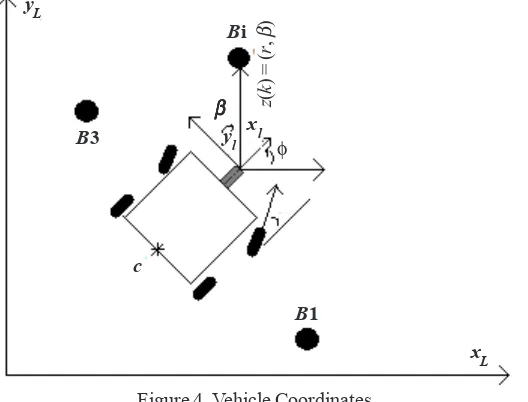
We represented the vehicle position in global coordinates as shown in figure 4 below. This model contains several parameters; the steering control α, which is defined in vehicle coordinate frame. We used laser sensor in the model and mounted it in the front of the vehicle. The landmarks are labeled as Bi(i = 1...n) and calculated based on the vehicle coordinates (x1, y1), where we have z(k) = (γ, β, I), where γ the distance from the beacon to the laser is and β is the sensor readings, considering vehicles coordinate frame, and I is the intensity information.
Figure 4. Vehicle Coordinates
Suppose that the vehicle is controller through the vehicle velocity vc and the steering angle α. Then to predict the trajectory of the back axle center C, we should follow the below equation.
χc
Yc
φc
Vc . cos(φ)
Vc . sin(φ)
Vc L . tan(α)
⎣
⎡
⎤
⎦
⎣
⎡ ⎤
⎦
=Because the laser is located in the front of the vehicle, the translation of the center of the back axle can be given:
Pl = Pc + a.Tθ + b. Tφ + π2
The transformation is defined by the orientation angle, according to the following vector Tφ expression:
→ ⎯→
B1 B3
c
Bi
xL yl xl
βββββ z(k
) = (
r
,
β
)
yL
Tθ = (cos (φ). sin(φ)) →
Where the scalar representation of the above equations is:
χl = χc + a. cos (φ) + b. cos(φ + )π2
Yl = Yc + a. sin (φ) + b. sin(φ + )π2
The velocity is generated by the encoder and translated to the center of the axle, as the equation:
Finally, the full state is represented as:
χL
YL
φL
Vc . cos(φ) −
Vc L . tan(α)
⎣
⎡
⎤
⎦
⎣
⎡ ⎤
⎦
= VcL (a. cos (φ) + b. cos(φ )). tan (α) Vc . sin(φ) − Vc
L (a. cos (φ) −b. sin(φ )). tan (α)
Vc = Vc
1−tan(α).
L H Where H and L given and represent the characteristics of the car.
The discrete vehicle and sensor model in global coordinates could be approximated as:
χk Yk φk
⎣
⎡ ⎤
⎦
=x (k − 1) + ∆tVc(k − 1). cos (∅(k − 1) −Vc
L (a. sin φ (k −1) + b. cos (φ (k −1))). tan (α) (k −1)) y (k − 1) + ∆tVc(k − 1). sin (∅(k −1) +Vc (k −1)(a. cos φ (k −1) + b. sin (φ (k −1))). tan (α) (k −1))
L Vc (k −1)
L . tan (α) (k −1)
⎤
⎦
⎣
⎡
The previous process can be approximated as a nonlinear equation:
X (k) +f (X (k − 1), µ (k − 1)) + ωc(k − 1) + ωf (k − 1)
Where X (k −1) and u (k −1) is the estimate and input at time k −1 and m (k −1) and wc(k −1) is: [ωµ(k) ] = [∆fµ(k −1) (X, µ)] µ(k)
∆fµ=∂∂µf
∂(µ1, µ2) ∂(x, y, φ) =
Which is the gradient of considering the input u (u1, u2) = (v, α) and µ(k) is the Gaussian noise (Chin12).
To observe the states using the equation:
Zr Zβββββ
i
i
⎦
⎤
⎡
⎣
= h(X, xi , yi ) =(xL −xi )2 + (y
L −yi )2
(xL −xi ) (yl −yi )
atan
⎛
⎝
−θ +π2⎠
⎞
⎣
⎡
⎤
Where z and [x, y, φ ] are the observation and state values respectively, and (xi , yi) are the positions of the beacons or the true landmarks. The observation representation can be shortened as:
z [k] = h (x(k)) + η (k)
Where η (k) is:
η (k) = ηR (k)
ηβ (k)
⎣
⎡
⎤
⎦
The Gaussian noises µ (k) and η (k) are temporarily uncorrelated and zero mean, as follows: E [µ (k)] + E [η (k)] = 0
With covariance:
E [µ (i)µ T ( j)] = δ
ijδα, v ( j), E [η (i)η T ( j)] = δijRγ, β( j) 4.2 Map Building
In our method, we used Back-propagation Artificial Neural Network (ANN) to make the robot estimate the locations of landmarks. In our case, we trained the ANN on the SLAM landmark equation results and the true landmarks from the dataset. Initially the vehicle starts at an unknown position with predefined uncertainty and obtains measurements using the ANN relative to its position. The ANN output and the sensor information are used together to incrementally build and maintain a navigation map and localization respecting the map.
The state vector is:
X = χv
χL
⎣
⎡ ⎤
⎦
Xv = [χ ,Y, φ ] ∈ R3 XL = [χ1, y1,... ..., χn, yn] ∈ RNWhere χv and χl are the states of the vehicle and the real landmarks. The ANN model of the extended system that considers the new states is:
f (x) = sign (w, x) + b = sign b +
∑
n
i = 1 wi xi
⎛
⎝
⎠
⎞
Where x is the state vector xv and xLfor static landmarks:
χv(k + 1) = f (χv(k))
χL(k + 1) = χL(k)
The Jacobian matrix for this system is:
∂F
∂X
∅T
= ∂f
∂χv =
⎣
⎡
J∅1T ∅ I⎤
⎦
⎣
⎡ ⎤
⎦
J1∈R3*3, ∅∈R3*N, I ∈RN *N
Then the observations are relative to the vehicle position. They can be represented as a function of vehicle state and the ANN output, which is the landmark positions.
ri = hr (k) = || (x, Y ) − (xi −yi ) ||2 = (xL −xi )2 + (y
l −yi )2
(xL −xi ) (yl −yi )
2
−θ +π
⎛
⎝
⎠
⎞
Where (x, y) is the position of the vehicle, (xi yi ) are the vector output of the ANN, which represent the landmark positions given i , and φ is the vehicle orientation. The Jacobian matrix of the vector (ri ,αi ) with respect to the variables (x, y, φ,xi yi ) can be calculated using:
∂h
∂X=
∂hr
=
⎣
⎡ ⎤
⎦
∂X∂hα
∂X
∂ri
∂(x, y, φ, {xi yi}) ∂αi
∂(x, y, φ, {xi yi})
⎤
⎦
⎣
⎡
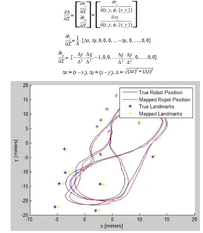
And∂hr
∂X
∂hα
∂X
=∆1. [∆x, ∆y, 0, 0, 0, .... −∆y, 0, ..., 0, 0]
=. [ −
∆x = (x − xi), ∆y = (y − yi), ∆ =
∆y
∆2,
∆χ
∆2, − 1, 0, 0, ....
∆y
∆2,
∆y
∆2, 0, ..., 0, 0]
(∆x)2 + (∆y)2
Using these equations, the robot can build and maintain a navigation map of the environment and track its position.
After explaining our approach and methodology, in addition to our experiment and evaluation of this approach, in the next section we will show our obtained results and discuss them.
4.3 Results and Discussions
In this experiment, it is used a dataset contains the true landmarks and GPS coordinates for our map were taken from Drexel Autonomous System Lab datasets, which where scanned using SICK scanner [23] , the researcher used the vehicle model and sensor pose, mentioned earlier. The researcher evaluated his algorithm using MATLAB® R2013a. The resulted map is shown in the below figure.
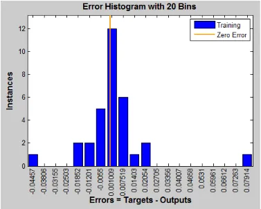
Figure 6. ANN Model Error Histogram
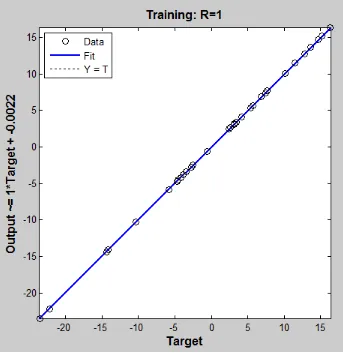
Figure 8. Regression Plot
The performance plot is shown in figure 7.
The regression plot for the model is shown in figure 8.
The uncertainty in the position becomes significantly smaller than the SLAM with beacons only or the SLAM with natural features. This is due to the use of ANN, which trained a larger number of landmarks that incorporate more information to the Kalman filter. From the error histogram and the plots above, the researcher can notice that we have reached good results of landmarks mapping which is very close to the true landmarks position. Based on that, we have obtained very good results of environment mapping, as shown in figure 5 above, the model mapped line is very close with the true line.
5. Conclusions
In this work, the researcher represented a new Simultaneous Localization and Mapping algorithm based on Artificial Neural Network, which resulted in high accuracy navigation and mapping. The design of this algorithm, in addition to the modelling aspect are presented with an implementation of it. Modeling SLAM using landmarks does not require any landmarks surveying. The results showed that the use of these landmarks in the ANN could deliver an accuracy considering the initial vehicle uncertainty. The obtained maps are relative to the initial coordinates of the vehicle, which gives more reliability to the resulted maps. In case of using GPS, we it is noticed that, the vehicle uncertainty needs to be incorporated.
References
[1] Smith, R., Cheesman, P. (1987). On the representation of spatial uncertainty. Int. J. Robotics Research, 5 (4) 56-68. [2] Durrant-Whyte, H. F. (1988). Uncertain geometry in robotics. IEEE Trans. Robotics and Automation, 4 (1), 23-31.
[3] Zhang, Xinzheng, Ahmad B. Rad, Yiu-Kwong Wong. (2012). Sensor fusion of monocular cameras and laser rangefinders for line-based simultaneous localization and mapping (SLAM) tasks in autonomous mobile robots. Sensors, 12 (1) 429-452. [4] Engelhard, Nikolas, et al. (2011). Real-time 3D visual SLAM with a hand-held RGB-D camera. In: Proc. of the RGB-D Workshop on 3D Perception in Robotics at the European Robotics Forum, Vasteras, Sweden.
[5] Gil, Arturo, et al. (2010). A comparative evaluation of interest point detectors and local descriptors for visual SLAM. Machine Vision and Applications, 21 (6) 905-920.
[6] Leonard, J. J., Durrant-Whyte, H.F. (1991). Simultaneous map building and localization for an autonomous mobile robot. In: Proc. IEEE Int. Workshop on Intelligent Robots and Systems (IROS), p. 1442-1447, Osaka, Japan.
[7] Sola, Joan, et al. (2012). Impact of landmark parametrization on monocular EKF-SLAM with points and lines. International Journal of Computer Vision, 97 (3) 339-368.
[8] Carrillo, Henry, Ian Reid, José A. Castellanos. (2012). On the comparison of uncertainty criteria for active SLAM. Robotics and Automation (ICRA), 2012 IEEE International Conference on. IEEE.
[9] Durrant-Whyte, H., Rye, D., Nebot, E. (1996). Localisation of automatic guided vehicles. In: G. Giralt, G. Hirzinger, editors, Robotics Research: The 7th International Symposium (ISRR’95), p. 613-625. Springer Verlag.
[10] Cheein, Fernando A. Auat, Ricardo Carelli. (2011). Analysis of different feature selection criteria based on a covariance convergence perspective for a SLAM algorithm. Sensors (Basel, Switzerland) 11(1) 62.
[11] Dissanayake, Gamini, et al. (2012). Convergence comparison of least squares based bearing-only SLAM algorithms using different landmark parametrizations .
[12] Benini, A., et al. (2011). Adaptive extended kalman filter for indoor/outdoor localization using a 802.15. 4a wireless network. In: Proceedings of the 5th European Conference on Mobile Robots ECMR.
[13] Kümmerle, Rainer, et al. (2011). Large scale graph-based SLAM using aerial images as prior information. Autonomous Robots, 30 (1) 25-39.
[14] McDonald, John, et al. (2011). 6-DOF multi-session visual SLAM using anchor nodes. European Conference on Mobile Robotics, Orbero, Sweden. V. 13.
[15] Lee, Yong-Ju, Jae-Bok Song, Ji-Hoon Choi. (2012). Performance Improvement of Iterative Closest Point-Based Outdoor SLAM by Rotation Invariant Descriptors of Salient Regions. Journal of Intelligent & Robotic Systems, p. 1-12.
[16] Mei, Christopher, et al. (2011). Hidden view synthesis using real-time visual SLAM for simplifying video surveillance analysis. Robotics and Automation (ICRA), IEEE International Conference on. IEEE.
[17] Stachniss, Cyrill, Stefan Williams, José Neira. (2010). Editorial: Visual navigation and mapping outdoors. Journal of Field Robotics, 27 (5) 509-510.
[18] Lee, Yong-Ju, Joong-Tae Park, Jae-Bok Song. (2011). Three-dimensional outdoor SLAM Using rotation invariant descriptors of salient regions. Control, Automation and Systems (ICCAS), 11th International Conference on. IEEE.
[19] Dissanayake, M. W. M. G., Newman, P., Durrant-Whyte, H. F., Clark, S., Csobra, M. (1999). An experimental and theoretical investigation into simultaneous localization and map building (SLAM). In: Proc. 6th International Symposium on Experimental Robotics, p. 171-180, Sydney, Australia, March.
[20] Definition according to openslam.org, a platform for SLAM researchers.
[21] Berns, Karsten, Ewald von Puttkamer. (2009). Simultaneous localization and mapping (SLAM). M.W.M.G. Autonomous Land Vehicles. Vieweg+ Teubner, p. 146-172.