A New Parallel Matrix Multiplication Method
Adapted
o
n Fibonacci Hypercube Structure
L. Jokar
*Department of Computer,Faculty ofComputer and Sciences, Islamic Azad University ofRodehen, Rodehen, Islamic Republic of Iran
Received: 24 August 2009 / Revised: 2 February 2010 / Accepted: 6 April 2010
Abstract
The objective of this study was to develop a new optimal parallel algorithm for
matrix multiplication which could run on a Fibonacci Hypercube structure. Most
of the popular algorithms for parallel matrix multiplication can not run on
Fibonacci Hypercube structure, therefore giving a method that can be run on all
structures especially Fibonacci Hypercube structure is necessary for parallel
matrix multiplication. For creating this method, a new model for matrix
multiplication with an algorithm for data distribution on Fibonacci Hypercube
structure was provided. Other than this, another optimized algorithm was designed
on Mesh structure. By running the algorithms on a simulative parallel system and
giving the results in graphical mode, it has been found that these two algorithms
have optimized value in parallel matrix multiplication and they are more efficient
than the previous algorithms.
Keywords: Broadcast; Cost-Optimal; Fibonacci Hypercube; Matrix multiplication; Parallel
* Corresponding author, Tel.: +98(21) 22336330, Fax: +98(21) 22336330, E-mail: [email protected]
Introduction
It seems somewhat strange to be writing a paper on parallel matrix multiplication almost three decades after commercial parallel systems first became available, one would think that by now we would be able to manage such an apparently straight forward task with simple, efficient implementations and a new method. This paper appears to have gained a new insight into this problem.
In the last three decades, numerous parallel algorithms were implemented for the matrix multiplication. The most common parallel matrix multiplication algorithms are Fox's algorithm, Cannon's algorithm, Strassen's algorithm [1,6,9] and parallel algorithms which were designed to run on Mesh and
the Fibonacci Hypercube structure recommended by Anisimov [2]. Anisimov proved that the Fibonacci Hypercube has the same property as Hypercube but with fewer connectors plus the same number of vertices.
With regard to the specification of structure which Fibonacci Hypercube has, not every method that was previously presented for the parallel matrix multiplication will be applicable on this structure. In 2006, Jokar and Ahrabian with regard to various dimension sizes of matrixes have presented and performed two algorithms(panel_dot and panel_block algorithms) which according to the existing method on this structure was possible to execute [13]. In this article with regard to various sizes of matrices has been presented a new method for parallel matrix multiplication that in addition is able to perform on every parallel structure and can also be performed on Fibonacci Hypercube. This research provides a new algorithm, based on this new method on Fibonacci Hypercube structure and shows that this algorithm is cost-optimal.
At the end of this research, some theoretical and experimental results have been provided. Also the results of execution of algorithm on the mesh and Fibonacci Hypercube structures and the comparison of various execution algorithms against each others were produced. It has been found that these two algorithms have optimized value in parallel matrix multiplication and they are more efficient than the previous algorithms.
The Fibonacci Hypercube Structure
The Fibonacci Hypercube was introduced by Anisimov [2] initially in 1997. This Fibonacci Hypercube is a new topological structure that is obtained recursively using formulas similar to the relation of Fibonacci numbers. It has properties very close to the Hypercube. In this part a very brief explanation is given:
Assume that we have p processors p p0, ,...,1 pP-1, knowing that p is a Fibonacci number and for each processor a binary index is attributed which the binary representation of numbers is substituted by the representation of numbers by sums of Fibonacci numbers. Each processor will be connected to the vertices that their index differ by just in one position. They called this structure the Fibonacci Hypercube. In this structure, the number of bits which form the index of vertices is called dimension. We assume that the
, F n
C shows a Fibonacci Hypercube with a number of
2 n
f + vertices which in that index, each vertex can be
shown with n bit. Fibonacci Hypercube with n dimension can be presented as n-Fibonacci Hypercube.
If we show the connections of the processors as a graph, therein the set of all edges in CF n, presented as
n
E and the set of all labels of vertices of CF n, structure presented as FCn, Also the number of vertices of CF n, can be presented by FCn .
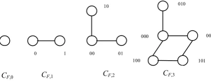
In Figure 1, Fibonacci Hypercubes CF,0, CF,1, CF,2, ,3
F
C are depicted.
Properties of the Fibonacci Hypercube 1st Property:
1 0 10 1
n n n
FC + = FC + FC - . (1) 2nd Property:
1 1 2
0 010
n k k n k n
FC + =FC FC - +FC - FC - . (2) 3rd Property: Number of vertices of
, F n
C is equal to
2 n
f +
4th Property:If a and b are adjacent vertices in
, F n
C then H a b( , ) 1= (is the hamming distance between a and b)[12] and if ,a bÎFCn and H a b( , ) 1= then a
and b are the adjacent vertices in CF n, .
Data Decomposition
For simplicity, we will assume that the dimensions m, n and k are integer multiples of the algorithmic block size b. When discussing this algorithm, we use the following partitionings A, B and C :
0
1 1
ˆ
ˆ
( )
ˆ
x
x
n b
n b
X
X
X X X X
X
æ ö
ç ÷
ç ÷
ç ÷
= =
ç ÷
ç ÷
ç ÷
è ø
o L M . (3)
where X Î
{
A B C, ,}
and mx and nx are the row andcolumn dimension of the indicated matrix.
Figure 1. Fibonacci Hypercubes CF,0, CF,1, CF,2, CF,3.
0 1 00 01
10 010
000
100 101
00
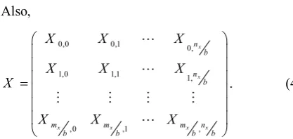
Also,
0,0 0,1 0,
1,0 1,1 1,
,0 ,1 ,
x
x
x x x x
n b
n b
m m m n
b b b b
X X X
X X X
X
X X X
æ ö
ç ÷
ç ÷
ç ÷
=
ç ÷
ç ÷
ç ÷
è ø
L L
M M M M
L
. (4)
In the above partitioning, the block size b is chosen to maximize the performance of the local matrix- matrix multiplication operation.
Vector Based Matrix Distribution
It is more natural to start by distributing the problem to nodes, we partition vector x and assign portions of this vector to nodes. The matrix A is then distributed to nodes so that it is consistent with the distribution of the vectors, as we describe below.
Assume that we have p processors. We use the following partitioning
0
1
1 p
x x x
x -æ ö ç ÷ ç ÷ = ç ÷ ç ÷ ç ÷ è ø
M . (5)
This vector is distributed by assigning xi to Pi. We
call such matrix distribution, vector based.
Broadcasting a Datum to Fibonacci Hypercube Architecture
We broadcast a datum to Fibonacci hypercube CF n, with O n( ) time complexity that n is Fibonacci hypercube dimension. According to the first property and structure of Fibonacci Hypercube the following identities for time complexity can be obtained:
, , 1 , 2
,0
, ,0
, ,0
( ) ( ) 1 ( ) 2
... ( )
( ) ( )
( ) ( ). ( ) 1
F n F n F n
F
F n F
F n F
T C T C T C
T C n
T C T C n
T C O n
T C
-
-= + = +
= = +
= + ü
Þ =
ý
= þ
For example:
For (n=10) CF,10 Þf12=144 (number of
processsors is 144).
The algorithm for broadcast to CF n, is as follows: Broadcast_Fib_H(n,x)
{
If P0 did not receive the data then P0¬x ; If n=0 Return();
If n=1 then P0 Send Data to P1; Else
{ // adjacent function returns the adjacent processor
0
P that is in bit nth differ.
P0 Send Data to adjacent(P0,n) ; do in parallel
{
Broadcast_Fib_H(n-1,x); //Do in parallel Broadcast_Fib_H(n-2,x); //Do in parallel }
} }
Figure 2. Broadcasting algorithm in Fibonacci Hypercube
CF,n.
Gathering Operation
In gathering operation, each processor stores its own data in the shared-memory.
The algorithm for gathering to ˆCh be as follows:
Gather ( ˆCh) {
For i =0 to P-1 do in parallel Pi Write ( )C i to Ch i,
}
Figure 3. Gathering operation in shared-memory.
Model of Communication Cost
We will assume that in the absence of network conflict, sending a message of length n between any two nodes can be models by:
s w
t +nt . (6)
Where ts represents the latency (startup cost) and tw represents the cost per byte transferred.
Parallel algorithm In this part, an optimal parallel algorithm is given for the matrix multiplication. It was mentioned in the previous article[13], two algorithms which according to the existing method on this structure was possible to execute have been presented. There have been showed that one of these algorithms in
1
1 n 2
is in k ffn f1 n1+2 also is cost-optimal. In this section with regard to various sizes of matrices a new method for parallel matrix multiplication that in addition is able to perform on every parallel structure and can also be performed on Fibonacci Hypercube has been presented. Here we present a new algorithm, based on this new method on Fibonacci Hypercube structure and show that this algorithm in nffn f1 n1+2 is cost-optimal. Also
show that this algorithm will be applicable on mesh structure.
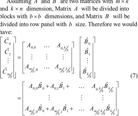
Matrix-Matrix Multiplication Bbased on Block-Panel Assuming A and B are two matrices with m k´ and k n´ dimension, Matrix A will be divided into blocks with b b´ dimensions, and Matrix B will be divided into row panel with b size. Therefore we would have:
0 0
0,0 0,
1 1
,0 ,
0,0 0 0,1 1 0,
0 1
,0 ,1 ,
ˆ ˆ
ˆ ˆ
ˆ ˆ
ˆ ˆ ˆ
ˆ ˆ ˆ
k b
m m k
b b b
k m
b b
k k
b b
m m m k k
b b b b b
C A A B
B C
A A
B C
A B A B A B
A B A B A B
é ù é ù
é ù
ê ú ê ú
ê ú
ê ú ê ú
= ê ú
ê ú ê ú
ê ú
ê ú ê ú
ê ú
ê ú ë û ê ú
ê ú
ê ú ë û
ë û
é + + ù
ê ú
ê ú
=
ê ú
ê + + ú
ë û
K
M M M M
M
K
K
M M M
K
(7)
This method is designed based on multiplication of blocks of A by row panels of B .This method is called multiplication of block-panel. In this method, from the sum of multiplication of block of ith row of matrix A by the row panels of matrix B , row panel
ˆ
i
C of matrix C will be obtained.
Parallel Matrix Multiplication Algorithm on a Fibonacci Hypercube
If we consider CF n,1 Structure, as we know the
number of processors in this structure is fn1+2 that n1 is Fibonacci Hypercube dimension.These nodes are connected through som communication network, which could be a Fibonacci hypercube (Intel 2.8 full cash).
This algorithm is designed based on multiplication of block-panel.
In this algorithm the following steps will be repeated by mb´kb times.
1) A block from matrix A, will be distributed in
every processor.
2) Members of panel ˆBs will be distributed amongst all the processors in a vector based method.
3) The result of ( )C i =C i( )+A i( )* ( )B i will be computed by every processor simultaneously.
4) After the steps 1 to 3 repeated by kb times. In gathering operation, a panel of matrix C will be computed.
Algorithm procedure is shown as follows: Procedure Fib- block-panel -Multip(A,B ,C ) Begin
For h=0 to m b Do
Begin
For i =0 to fn1+2 Do in Parallel ( )C i ¬0;
For s=0 to k b Do
Begin
Broadcast_Fib(n A1, h s, )
For i =0 to fn1+2 Do in Parallel
B i( )¬Bs i, ;
For i =0 to fn1+2 Do in Parallel ( )C i =C i( )+A i( )´B i( ); End;
Gather to ˆCh; End;
End.
Figure 4. block-panel Algorithm in
1
, F n
C structure.
Cost-Optimality: The first step of algorithm takes
2 1
(ts +b t nw) time. In the second step of algorithm, ˆBs in the constant time will be distributed amongst all the processors in the vector based method. In the third step, the multiplication of two matrices with the dimensions of b b´ and
1 2
n
n b
f +
´ will be computed by all the processors simultaneously. Therefore, this multiplication takes 2
1
( )
2
n b
1
1
2 2
1
2
1
2
( (( ) ))
( ).
P s w
n
w n
k m n
T O b b t b t n f b
knm O kmn t
f
+
+
= * + + *
= + (8)
Then cost of algorithm will be equal to:
1
1 2
( ).
P n
Cost T= * =P O kmn f + +knm (9) We know the condition of cost -optimality is:
(1). *
Seq
P
T
E O
P T
= = (10)
Therefore to have cost -optimal algorithm we must have:
1
1
1 2
1 2 .
n
n
kmn f knm
n f n
+
+
Þ
pp
pp (11)
Therefore, for the case where n f1 n1+2 ppn the algorithm is cost-optimal.
Parallel Matrix Multiplication Algorithm on a Mesh As mentioned, this method for parallel matrix multiplication is able to perform on every parallel structure. In this section, we present the block-panel algorithm that designed to run on a mesh. For presented algorithm, we will assume a logical r c´ mesh of computational nodes which are indexed Pi j, 0£ <i r and 0£ <j r , so that the total number of processors is
p= ´r c. These nodes are connected through some communication network, which could be a higher dimensional mesh (Intel 2.8 full cash).
This algorithm is designed based on multiplication of block-panel.
In this algorithm the following steps will be repeated by mb´kb times.
1) A block from matrix A, will be distributed in every processor.
2) Members of panel ˆBs will be distributed amongst
all the processors in a vector based method.
3) The result of ( )C i =C i( )+A i( )* ( )B i will be computed by every processor simultaneously.
4) After the steps 1 to 3 repeated by kb times. In gathering operation, a panel of matrix C will be computed.
Algorithm procedure is shown as follows:
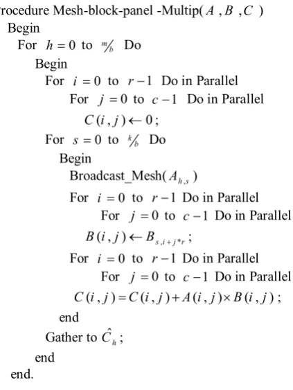
Procedure Mesh-block-panel -Multip(A,B ,C ) Begin
For h=0 to m b Do
Begin
For i =0 to r-1 Do in Parallel For j =0 to c-1 Do in Parallel ( , )C i j ¬0;
For s=0 to k b Do
Begin
Broadcast_Mesh(Ah s, )
For i =0 to r-1 Do in Parallel For j =0 to c-1 Do in Parallel B i j( , )¬Bs i j r, + * ;
For i =0 to r-1 Do in Parallel For j =0 to c-1 Do in Parallel ( , )C i j =C i j( , )+A i j( , )´B i j( , ); end
Gather to ˆCh;
end end.
Figure 5. block-panel Algorithm in Mesh structure.
Cost-Optimality: The first step of algorithm takes
2
(ts +b tw) logP time. In the second step of algorithm, ˆBs in the constant time will be distributed amongst all the processors in the vector based method. In the third step, the multiplication of two matrices with the dimensions of b b´ and b n
p
´ will be computed by all the processors simultaneously. Therefore, this multiplication takes ( *b2 n )
P time. The fourth step takes constant time. There are kb´mb iterations of steps 1 to 4 [12]. Thus, the algorithm time complexity is equal to:
2 2
( (( ) log * ))
( log ).
P s w
w
k m n
T O b b t b t P b P
knm O km Pt
P
= * + +
= + (12)
Then cost of algorithm will be equal to:
( log ).
P
(1). *
Seq
P
T
E O
P T
= = (14)
Therefore to have cost-optimal algorithm we must have:
log
log .
kmP P knm
P P n
Þ
pp
pp (15)
Therefore, for the case where PlogP ppn the algorithm is cost-optimal.
Results
This section reports the performance of algorithms that we presented in previous sections, on a system with 8 nodes.
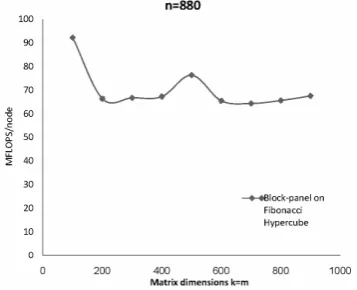
In Figure 6, we show the performance of parallel matrix multiplication algorithm based on block-panel that are designed to run on CF,4. For the case where
1
1 n 2
n>>n f + , this algorithm is cost-optimal. The results for the case where n dimension is fixed and large have been presented. It is clear from the graph (in accordance to the Figure 6) that to increase dimension of k and m in comparison to the dimension of n, the speed of performance of algorithm will be reduced. Therefore, if dimension of n is fixed and large this algorithm will be an improved algorithm.
In Figure 7, we show the performance of parallel matrix multiplication algorithm based on block-panel that are designed to run on a 4 2´ Mesh. Considering, for the case where n>>plogp, this algorithm is cost-optimal, we present results for the case where n dimension is fixed and large. It is clear from the graph (in accordance to the Figure 7) that to increase dimension sizes of matrixes, the speed of performance of algorithm will be increased. Therefore if dimension sizes of matrixes are large this algorithm will be an improved algorithm.
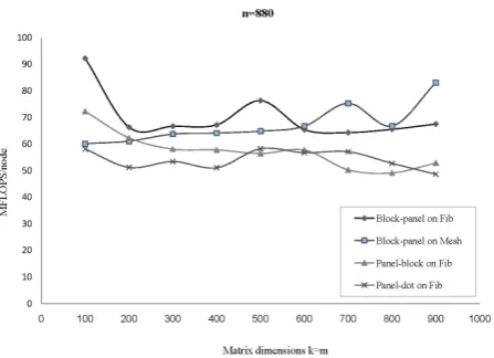
In Figure 8, the results of execution of panel-dot and panel-block algorithms which have designed to run on
,4 F
C [13] and block-panel algorithm were compared. The results for the case where n dimension is fixed and large have been presented. It is clear from the graphs (in accordance to the Figure 8) that the block-panel algorithm has a better performance time in respect to the other two algorithms (panel-dot and panel-block algorithms)[13]. Also, for all points the performance time of block-panel algorithm on the Fibonacci hypercube structure is best.
Discussion
The main drawback of the hypercube structure is the necessary increase of each vertex valence while increasing a hypercube dimension. This means that the value of the communication hardware grows faster than a hypercube dimension. Taking into consideration that a higher number of Hypercube and higher dimensional mesh will lead to a considerable rise in the number of connections of processors and consequently this will lead to a fast growth in the hardware. By using the presented algorithm in the Fibonacci Hypercube Structure the cost of Connection amongst the processors will be reduced (because the Fibonacci hypercube
Figure 6. Performance of parallel matrix multiplication algorithm based on block-panel that designed to run on CF,4.
Figure 8. Performance of various parallel matrix multiplication algorithms.
structure has the same property as hypercube structure but with fewer connectors plus the same number of vertices).
The block- panel algorithm is designed to run on 1
, F n
C structure. As we know the number of processors in this structure is fn1+2, where n1 is Fibonacci
hypercube dimension. As shown in the previous sections, the time complexity of this algorithm is
1
1
2
( w )
n
knm o kmn t
f +
+ and for the case where n>>n f1 n1+2, this algorithm is cost-optimal. In accordance to the procedure of this algorithm, the steps of algorithm will be repeated by m k 2
b
* times; therefore, if the
dimension of n is fixed and large, this algorithm would have a better performance time in comparison to the panel-dot and panel-block algorithms.
As mentioned, this method for parallel matrix multiplication is able to perform on every parallel structure. In this research, the block-panel algorithm is designed to run on a logical r c´ mesh of computational nodes which could be a hypercube (a higher dimensional mesh).As shown in the previous sections, the time complexity of this algorithm is
( log w )
knm o km pt
p
+ and for the case where log
n>>p p, this algorithm is cost-optimal. In accordance to the procedure of this algorithm, the steps of algorithm will be repeated by m k 2
b
* times;
therefore, if the dimension of n is fixed and large, this algorithm would have a better performance time in
comparison to the panel-dot and panel-block algorithms. Comparing the graph of the charts in the Figures 6 and 7 it can be said in the points where k <600,
600
m< , the speed of performance of block-panel algorithm on Mesh structure has a better performance time than this algorithm on Fibonacci Hypercube structure. Also, in these points, this algorithm on Mesh is best.
As it is seen in the Figure 8, in all points the block-panel algorithm will take less time and has a better performance time in respect to the other two algorithms (panel-dot and panel-block algorithms).
References
1. Akl S.G., The design and Analysis of Parallel Algorithms,
Queens University, Prentice, Hall International, Inc, (1989).
2. Anisimov A.V., Fibonacci Hypercube, International
Journal of compute mathematics, 25: 221_227 (1997).
3. Benner P., E.s, Ortf Q., Quintana G., Numerical Sedation
of Discrete Stable Linear Matrix Equations on
Multicomputers, Parallel Algorithms and Applications,
17(1):127-146(2002).
4. Chtchekanova A., Gunnels J., Morrow G., Overfelt J., geijn R., Parallel Implementatio of BLAS : General
Techniques for level3 Blas, TR_95_40, Department of
Compute Sciences, University of Texas, (1995).
5. Fatahalian k., Sugerman J., Understanding The Efficiency
of GPU Algorithm for Matrix-Matrix Multiplication,
Presented at Graphics Harware, (2004).
6. Fox G.C., Johnson M.A., Lyzenga G.A., Wotto S., J.K.
and Walker D.W., Solving Salmo Problems on
Concurrent Processors, Prentice Hall, Englewood cliffs,
N.J.1(1) (1998).
7. Geijn R.V., Using PLAPACK : Parallel Linear Algebra
Package, The MIT Press, (1997).
8. Geijn R., Scalable Universal Matrix Multiplication
Algorithms, Concurrency : Practice and Experience,
9(4): 255_274(1995).
9. Grayson B., Pankaj S.A., Geijn R., A High Performance
Strassen Implementation, June13, (1995).
10. Gunnels J., Lin C., Morrrow G., Geijn R., Analysis of a
Class of parallel Matrix Multiplication Algorithms, A
Technical Paper Submitted to IPPS 98, (1998).
11. Jadish J.M., Parallel Algorithms and Matrix
Computation, University of Cambridge, Clarn Don Pess.Oxford, (1998).
12. Jokar L., Parallel Algorithms for Matrix Multiplication,
M.S Thesis, Department of mathematics and computer science, Tehran university, 172 p.(2002).
13. Jokar L., Ahrabian H., Optimal Parallel Matrix
Multiplication Algorithms on a Fibonacci Hypercube Structure, International Journal of Science & Technology Amirkabir, 17(64): 11-17(2006).
14. Maniezzo D., Villa G., Gerla M., A Smart Mac-Routing
Protocol for Wlan Mesh Networks, UCLA-CSD Technical