Which OIC countries are catching up? Time Series Evidences with Multiple Structural Breaks

Which OIC countries are catching up? Time Series Evidences with Multiple Structural Breaks

Zahra Elmi

Economics Faculty, Mazandaran University, Babolsar

[email protected]

Omid Ranjbar

Department of International Affairs and Specialized Agencies, Ministry of Industry, Mine, and Trade,Tehran

[email protected]

Abstract

In this paper, income per capita convergence hypothesis is tested in selected OIC countries. For this purpose, we use the time series model and univariate KPSS stationary test with multiple structural breaks (Carrion-i-Silvestre et al. (2005)) over the period 1950-2008. The results show that most OIC countries could not catch up toward USA. Although because of some positive term of trade shocks, they experienced catching up process in some sub- periods, they did not have appropriate infrastructure as, they could not use these opportunities and escape lag deadlock.

Keywords: Income convergence; Catching up; KPSS stationary test; Multiple structural breaks.

JEL Classification: O1;O47; C32; C33

1. Introduction

The convergence hypothesis is one of the neoclassical growth theory outcomes that is defined as a tendency of countries towards equalization over time in term of per capita income. This model predicts that the substitution possibility and diminishing return for factors to force the economy to converge to the equilibrium capital and income level (Islam, 2003). Endogenous growth theory, launched by Romer (1986) and Lucas

(1988), has primarily focused on the convergence theory and challenged the strong cross-country implications of the neoclassical model. In the endogenous growth theory, investment embodies spillover effects which offset the tendency towards diminishing return. Therefore, initial differences may exist and grow without limits over time. In other words, the endogenous growth theory rejects the convergence hypothesis and hence it can be used to distinguish between the two leading approaches to economic growth, namely the neoclassical growth theory and endogenous growth theory (Huang, 2005). However, Romer (1996) finds that if income differentials result from technological differences, by following technological know-how from technologically advanced countries to developing countries, the poorer countries would grow faster than richer ones. Nevertheless, as noted by Aghion and Howitt (2009), only if the poor countries devote resource to innovation, they will be able to simply copy and adapt the new technology to local conditions and thus grow as fast as the rich countries. If a country fails to invest on innovation, it will stagnate while the rest of the world continues to advance.

As surveyed by Rassekh (1998) and Islam (2003), in empirical works on convergence hypothesis, researchers have used different notions of convergence such as absolute convergence, conditional convergence, and deterministic convergence. According to previously mentioned notions, three methodologies materialized which may be classified as follows: (a) cross-section approach, (b) time series approach, and (c) distribution approach. For example, cross-section and time series approaches investigate absolute and conditional notions of convergence hypothesis. Absolute convergence refers to the notion that economies will converge toward the same income per capita in the long run steady state, whereas, conditional convergence implies that the economies will converge to their own steady state. In most of the empirical works, in order to investigate the absolute and conditional convergence, researchers use

convergence-growth or �-convergence equation. According to the convergence-growth

OECD countries that have similar economic structures, while conditional convergence hypothesis has been accepted among a broader sample of economies. Due to the use of the cross-section dataset, Baumol (1986), Delong (1988), Barro (1991), and Barro and Sala-i-Maitin (1991, 1992,

1995) used the �-convergence equation. Nonetheless, the �-convergence

equation has been widely criticized in the literature. For example, Quah (1993) discussed that a negative correlation between income per capita growth rate regress and initial income per capita may be Galton fallacy.

Evans and Karras (1996) show that �-convergence equation is valid only

if the economies have the identical first–order autoregressive dynamic structures and all permanent cross-country differences are completely controlled for, which are very restrictive assumptions. Bernard and Durlauf (1996) show that conditional convergence is a weaker notion of convergence than time series convergence. They find that cross-section tests tend to spuriously reject the null of no convergence when economics have different long–run steady states and the failure to reject the no convergence null using time series tests can be due to transitional dynamics in the data.

Time series model of convergence hypothesis is examined by unit root tests. Hence, empirical validity of the hypothesis is dependent some how upon advances in econometrics of unit root tests. In empirical works, several unit root tests are used namely, Augmented Dicky Fuller (hereafter ADF), Phillips and Perron (1988) (hereafter PP), Zivot-Andrews (1992) (hereafter ZA), Lumsdaine and Papell (1997) (hereafter

LP), Lee and Strazicich (2003), and Carrion-i-Silvestre et al. (2005)

(hereafter CBL). In this paper, we used the CBL unit root test mainly due to its advantages compared to the other unit root tests for testing of convergence hypothesis. Whereas CBL stationarity test is KPSS type unit root test, hence, its null hypothesis is stationary, in other tests the null hypothesis is non-stationary. Thus, in CBL test, the convergence hypothesis is tested directly. In addition, in CBL test, we are able to control for structural breaks that affect on result of stationary tests.

As noted by Islam (2003), the distribution approach focuses on the dispersion of the per capita income among countries. Sigma convergence is one version of the distribution and calculated by the standard deviation. If the cross-country standard deviation of the per capita income decreases over time, it represents that there exists the sigma convergence.

the CBL stationarity test among the Organization of the Islamic Conference (OIC hereafter). The OIC has a membership of 57 states spread over four continents and is the collective voice of the Muslim world. Whereas, all membership of OIC are classified as developing countries, is it important to determine which OIC countries are catching up? The objective of this paper is to empirically examine the convergence hypothesis across the OIC member countries. For this end, first, the time series approach of convergence hypothesis are selected. Second, the time series model is tested by using the univariate stationary test with multiple structural breaks. Third by selecting USA as a leader with high-income per capita level, the convergence theory is tested. In particular, convergence towards the USA is considered as catching up towards higher balanced growth path and divergence from USA is considered as

falling into poverty trap. To the best of our knowledge, this study is the

first of its kind to utilize the univariate stationary test with multiple structural breaks to investigate the time-series properties of per capita real GDP for the OIC countries. This empirical study contributes to the field of empirical research by determining the break dates that affected the OIC countries catching up process. Also, it is able to determine the catching up or divergence process that occurred after any break.

The remainder of paper is organized as follow. Section 2 describes data and the econometric methodology used. The empirical results are discussed in the section 3, and conclusion is presented in the final section.

2. Data and methodology 2.1 Data

because they do not have data for all years of the period 1950-2008.

2.2 Methodology 2.2.1 Empirical model

In this paper, in order to test the convergence hypothesis, we first apply the CBL stationarity test to the differences of the logarithm per capita GDP level of each country with respect to the USA. This is a necessary condition for convergence or catching up hypothesis. After we identified the break dates in linear trend using stationary test, we were able to investigate the sufficient condition for the catching up process. For this end, we follow Tomljanovich and Vogelsang (2002) and Carrion-i-Silvestre and German-Soto (2009) and estimate the following equation for the OIC member countries that the null of stationarity is not rejected for them.

��� = � ��

���

���

���,�+ � ��

���

���

���,�+ �� (1)

In equation (1), RI is logarithm of relative per capita real GDP, t and

m are time and optimal number of breaks respectively. Respectively, DU and DT are dummy variables in order to control for structural breaks in

intercept and slope of linear trend. The ��_�,� and ��_�,� are defined as

the following:

��_��= �

1 ���������������< � ≤ ���

0 ��ℎ�����������������������

�

����= �

� − ��_���� ��������_���< � ≤ ��_�

0 ��ℎ�����������������������

�

Where ���is kth break date. According to Carrion-i-Silvestre and

German-Soto(2009), there has been catching up process "when the

coefficients of the parameters of each regime are significant at least at the

�_� > 0 or when �_� > 0 and��_� < 0. If both parameters of each regime have the same sign and are significant at least at the 10% level of significance, we conclude the divergence has occurred. If catching up process has occurred but both parameters are not significant, we have achieved the equilibrium growth. If catching up process occurred but only one of the parameters is significant, we conclude that weak catching up process has occurred and when both of them is same sign but only one of the parameters is significant, the weak divergence has occurred.

2.2.2 Econometric framework

The CBL stationarity test is adopted in the study due to its advantages that allows for break in intercept and trend. In this test, the data generation process under the null of stationary is based on following model:

��� = � + �� + � ��

�

���

���,�+ � ��

�

���

���,�+ �� (2)

In equation (2),��, T and m are intercept, linear trend and number of

breaks, respectively. The break dummy variables take the following values:

���� = �

1 ����> ��_�

0 ��ℎ�����������������������

�

��_��= �

� − ��� ����> ���

0 ��ℎ�����������������������

�

The test statistic is computed as Kwiatkowski et al (1992) test with multiple breaks:

LM(�) = �����_{� ��}

� �

(3)

� ���

Where S�_�is the partial sum of the estimated OLS residuals from Eqn.

(2). �� denotes a heteroskedasticity and autocorrelation consistent

estimate of the long –run variance of ��. �is the location of the breaks

on the��, hence that is important that we identify the location and the number of breaks correctly. CBL recommend using the Bai and Perron (1998) procedure that is based upon the global minimization of the sum of squared residuals (SSR) as follows:

����_�, … , ���_�� = ������_(���_�,…,���_�)��������, … , ����� (4)

The optimal number of breaks is selected by CBL criterion of Liu, Wu, and Zidek (1997). In this paper, the finite sample critical values are computed by Monte Carlo simulations using 100000 replications.

3. Results

In order to examine the convergence hypothesis toward the USA, first we test the stationarity of GDP per capita gap series by CBL stationarity test with multiple structural breaks. The number of structural breaks has been

selected using the modified BIC defined in Liu et al (1997). According to

Carrion-i-Silvestre and German-Soto (2009) the initial maximum number

of structural breaks that we allow in our set-up is ����_{=5. However, in}

some cases this maximum is achieved, so that in order to ensure that

there are no structural breaks left we increase ����_{�to 8.}

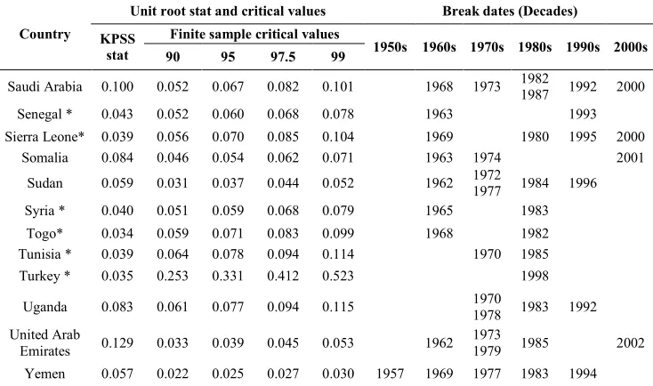
The results of test are shown in Table 1. As can be seen, the stationarity hypothesis is not rejected for Albania, Algeria, Bangladesh, Benin, Burkina Faso, Cameroon, Comoro Islands, Côte d'Ivoire, Gambia, Iraq, Lebanon, Mauritania, Morocco, Mozambique, Niger, Nigeria, Oman, Pakistan, Senegal, Sierra Leone, Syria, Togo, Tunisia, and Turkey. For these countries, the CBL stationary test’s statistic is statistically significance at the 10% level. For other countries, the CBL stationary test’s statistic is greater than the critical value at the 10% level; hence, the stationary hypothesis is rejected for them.

Break dates show all countries experienced at least one statistically significant structural break. This implies the importance of accounting for structural breaks in conducting tests for unit root. Distribution of breaks shows that they have occurred in all decades. Most breaks occurred in

1970sand 1980s. Respectively, 12, 34, 36, 41, 33, and 11 break points are

located around 1950s, 1960s, 1970s, 1980s, 1990s, and 2000s. As can be

procedure detects one country (Turkey) with one break, 12 countries with 2 breaks and respectively 3, 4, 5, 6, and 7 breaks for 10, 8, 6, 6, and 2 countries. Libya and Qatar present 7 break points in trending behavior.

Most of the OIC countries are highly specialized in the production and export of a few primary commodities. Hence, there is clear-cut evidence supporting the presence of clustering patterns of the break dates based on external shocks such as booms and busts of primary commodities prices. For example, the most oil exporting countries such as Iran, Iraq, Saudi Arabia, Bahrain, and Kuwait, experienced some breaks in level and slope of linear trend variable due to the oil booms of the period 1973-1974, 1979 and 2004 and a decrease in its price in the

mid-1980sand mid 1990s.

As mentioned by Romero-Avila (2009, pp:1059-1060), favorable terms of trade over the periods 1976-1979 and 1993-1994 and negative terms of trade shocks over most of the 1980 and 1990 (except 1993-1994) caused countries specialized in coffee such as Cameroon, Côte d'Ivoire, Sierra Leone, Uganda, and Togo to experience some positive and negative shocks in above dates. Regarding countries specialized in Cocoa such as Cameroon, Côte d'Ivoire, Sierra Leone, and Togo; there are evidences of positive breaks associated moderate increase in its price over 1960s. Cotton boom in the early and mid-1970s and the falling of its prices over the early 1980s caused the main cotton producers such as Pakistan, Sudan, and Guinea Bissau to experience some positive and negative breaks in their GDP's trending behavior.

In addition to the structural breaks associated with the terms of trade fluctuations, the military conflicts and wars took place in Afghanistan(2001), Algeria (1961), Bangladesh (1971), Egypt (1956 and 1973), Lebanon (1982), Iran (1981-1988), Iraq (1991), Mozambique (1974 and 1984), Nigeria (1966), Senegal (1992), Syria (1982-1985), Uganda (1978), and Yemen (1970) and revolution in countries such as Iran and Mozambique caused a sudden drop in the level of GDP per capita.

Country

Unit root stat and critical values Break dates (Decades)

KPSS stat

Finite sample critical values

1950s 1960s 1970s 1980s 1990s 2000s 90 95 97.5 99

Afghanistan 0.073 0.037 0.043 0.050 0.060 1963 1981 1994 2001 Albania * 0.021 0.030 0.034 0.037 0.041 1957 1973 1990 Algeria * 0.024 0.035 0.040 0.045 0.051 1961 1981 1996 Bahrain 0.189 0.019 0.021 0.023 0.026 1957 1966 1974 1981 1990 2000 Bangladesh* 0.035 0.066 0.083 0.100 0.123 1971 1990 2000

Benin * 0.032 0.107 0.138 0.168 0.212 1979 1987 Burkina

Faso* 0.037 0.038 0.044 0.050 0.058 1962 1972 1993 Cameroon * 0.019 0.037 0.044 0.051 0.060 1963 1980 ₁₉₈₆ 1993

Comoro

Islands * 0.038 0.070 0.085 0.099 0.119

1970 1979

Côte d'Ivoire* 0.022 0.037 0.043 0.048 0.056 1962 1982 1994

Djibouti 0.069 0.029 0.034 0.040 0.047 1961 ₁₉₆₉ 1976 1983 1998

Egypt 0.043 0.021 0.022 0.024 0.027 1955 1965 1974 1981 1994

Gabon 0.059 0.047 0.059 0.071 0.086 1967 1977 1986 1998 Gambia * 0.055 0.078 0.098 0.117 0.143 1973 1983

Guinea 0.041 0.040 0.047 0.053 0.061 1962 1974 1984

Guinea Bissau 0.068 0.065 0.078 0.091 0.109 1969 1997

Indonesia 0.043 0.025 0.029 0.034 0.041 1967 ₁₉₆₀ 1973 ₁₉₇₉ 1986 1997

Iran 0.025 0.019 0.021 0.023 0.025 1956 1967 1976 1981 ₁₉₈₉ 2002

Iraq * 0.024 0.034 0.039 0.044 0.050 1954 1978 1990

Jordan 0.133 0.018 0.020 0.022 0.024 1955 1964 1972 1981 ₁₉₈₈ 2002

Kuwait 0.078 0.020 0.022 0.025 0.028 1957 1969 1980 ₁₉₈₉ 1999 ₁₉₉₄

Lebanon * 0.053 0.133 0.172 0.211 0.264 1983 1990

Libya 0.022 0.016 0.017 0.018 0.020 1954 1962 ₁₉₆₉ 1974 1980 ₁₉₈₇ 1999

Malaysia 0.111 0.024 0.028 0.031 0.036 1959 1968 1981 ₁₉₈₇ 1997

Mali 0.028 0.027 0.030 0.032 0.036 1957 1974 1980 1993 Mauritania * 0.026 0.067 0.083 0.100 0.122 1971 1992

Morocco * 0.025 0.043 0.052 0.061 0.073 1965 1981 1998 Mozambique* 0.046 0.079 0.101 0.124 0.153 1974 1984 1994 Niger* 0.022 0.033 0.039 0.045 0.053 1962 1972 1983 2000 Nigeria* 0.017 0.044 0.055 0.065 0.079 1966 1973 1983 1998

Oman* 0.023 0.057 0.067 0.078 0.093 1967 1982 Pakistan* 0.093 0.107 0.137 0.170 0.213 1979 1997

Country

Unit root stat and critical values Break dates (Decades)

KPSS stat

Finite sample critical values

1950s 1960s 1970s 1980s 1990s 2000s 90 95 97.5 99

Saudi Arabia 0.100 0.052 0.067 0.082 0.101 1968 1973 1982 ₁₉₈₇ 1992 2000

Senegal * 0.043 0.052 0.060 0.068 0.078 1963 1993 Sierra Leone* 0.039 0.056 0.070 0.085 0.104 1969 1980 1995 2000

Somalia 0.084 0.046 0.054 0.062 0.071 1963 1974 2001 Sudan 0.059 0.031 0.037 0.044 0.052 1962 1972 ₁₉₇₇ 1984 1996

Syria * 0.040 0.051 0.059 0.068 0.079 1965 1983 Togo* 0.034 0.059 0.071 0.083 0.099 1968 1982 Tunisia * 0.039 0.064 0.078 0.094 0.114 1970 1985

Turkey * 0.035 0.253 0.331 0.412 0.523 1998

Uganda 0.083 0.061 0.077 0.094 0.115 1970 ₁₉₇₈ 1983 1992

United Arab

Emirates 0.129 0.033 0.039 0.045 0.053 1962 1973

1979 1985 2002

Yemen 0.057 0.022 0.025 0.027 0.030 1957 1969 1977 1983 1994

Notes: The finite sample critical values are computed by Monte Carlo simulation using 100000 replications. * denotes the stationarity hypothesis is not rejected at the 10% level.

In order to investigate the sufficient condition for the catching up process, we estimate the equation (1) for countries that the null of stationarity is not rejected for them. As mentioned in section 2.2.1, we denote respectively catching up, divergence, weak catching up, weak divergence, and equilibrium growth by C, D, c, d, and E hereafter. Table 2 reports the estimated coefficients of each of the m+1regimes and summarizes the different situations corresponding to each regime. In general, the results show that catching up process has taken part during the analyzed period, but the process has not been uniform in all regimes. For the first regime, there was catching up and divergence in 8 and 16 countries respectively. After first regime or first break, there was catching up process in 10 countries and divergence in 14 of 24 countries. For the third regime, there was catching up and divergence for 9 and 14 OIC member states respectively. There were six countries that show catching up process and six countries that show divergence process over forth regime. For the final regime, there was convergence process in three countries and one country that was diverged from the USA.

classification of OIC member countries

Country ��� ��� ��� ��� ��� ��� ��� ��� ��� ���

Albania 0.0150.005 -2.3060.000 -2.0980.000 0.0050.006 -1.9530.000 -0.0160.000 -2.6690.000 0.0340.000

C C D C

Algeria 0.0260.000 -2.0820.000 -2.0840.000 0.0150.000 -1.6810.000 -0.0400.000 -2.3040.000 0.0100.028

C C D C

Bangladesh

-0.015 -2.889 -3.423 -0.010 -3.577 0.003 -3.550 0.028 0.000 0.000 0.000 0.000 0.000 0.359 0.000 0.000

D D c C

Benin -0.0230.000 -2.2270.000 -2.7350.000 -0.0160.002 -2.9790.000 -0.0070.000

D D D

Burkina Faso 0.0130.000 -3.0550.000 -2.9560.000 -0.0060.086 -3.1660.000 -0.0080.000 -3.4260.000 0.0020.346

C D D c

Cameroon 0.0040.018 -2.6790.000 -2.7190.000 -0.0050.000 -2.6200.000 0.0200.015 -2.5980.000 -0.0820.000 -3.2460.000 0.0000.971

C D C D c

Comoro Islands

0.011 -2.887 -2.498 -0.108 -3.237 -0.028 0.000 0.000 0.000 0.000 0.000 0.000

C D D

Côte d'Ivoire 0.0060.010 -2.2740.000 -2.1020.000 -0.0070.000 -2.2990.000 -0.0650.000 -2.9320.000 -0.0320.000

C D D D

Gambia 0.0000.845 -2.7670.000 -2.6320.000 -0.0320.000 -3.2270.000 -0.0110.000

c D D

Iraq 0.1360.000 0.000 0.000 0.004 0.000 0.000 0.000 0.000 -2.174 -1.528 0.008 -0.903 -0.110 -3.032 -0.022

C C D D

Lebanon -0.0090.000 -1.4220.000 -1.6690.000 -0.1300.000 -2.1160.000 0.0050.118

D D c

Mauritania 0.0210.000 -3.1090.000 -2.7230.000 -0.0240.000 -3.2460.000 0.0030.239

C D c

Morocco

-0.024 -1.862 -2.304 0.010 -2.097 -0.012 -2.381 0.017 0.000 0.000 0.000 0.000 0.000 0.000 0.000 0.000

D C D C

Mozambique -0.004 -2.144 -2.463 -0.046 -3.090 0.002 -3.213 0.037 0.011 0.000 0.000 0.000 0.000 0.685 0.000 0.000

D D c C

Niger 0.009 -2.797 -2.578 -0.039 -3.227 0.005 -3.479 -0.036 -4.089 -0.008 0.001 0.000 0.000 0.000 0.000 0.148 0.000 0.000 0.000 0.115

C D c D d

Nigeria

-0.011 -2.492 -3.099 0.087 -2.409 -0.045 -3.021 -0.005 -3.244 0.020 0.000 0.000 0.000 0.000 0.000 0.000 0.000 0.093 0.000 0.001

D C D D C

Oman

0.024 -2.776 -1.462 0.002 -1.167 -0.009 0.000 0.000 0.000 0.648 0.000 0.000

C C D

Pakistan -0.0010.082 -2.8120.000 -2.7370.000 0.0060.000 -2.7760.000 0.0110.000

D C C

Country ��� ��� ��� ��� ��� ��� ��� ��� ��� ��� 0.667 0.000 0.000 0.000 0.000 0.924

d D c

Sierra Leone 0.001 -2.657 -2.591 -0.024 -2.713 -0.047 -3.760 -0.108 -4.070 0.034 0.514 0.000 0.000 0.000 0.000 0.000 0.000 0.000 0.000 0.000

c D D D C

Syria

0.005 -1.303 -1.546 0.033 -1.272 -0.003 0.234 0.000 0.000 0.000 0.000 0.212

C C d

Togo

0.012 -2.904 -2.566 -0.026 -3.106 -0.035 0.000 0.000 0.000 0.000 0.000 0.000

C D D

Tunisia

0.003 -2.177 -1.997 0.012 -2.003 0.014 0.074 0.000 0.000 0.000 0.000 0.000

C C C

Turkey

0.006 -1.691 -1.580 0.023 0.000 0.000 0.000 0.000

C C

Notes: C, c, D, and d denote catching up, weak catching up, divergence, and weak divergence, respectively.

4. Conclusion

One of the oldest controversies in the economic growth literature is Convergence hypothesis. According to the hypothesis, income per capita inequality will disappear in the long run. This paper examined the GDP per capita catching up process of selected OIC (36 countries) toward USA GDP per capita by time series model of convergence hypothesis and univariate stationarity test over period 1950-2008. Toward this end, we

used the Carrion-i-Silvestre et al. (2005) stationarity test that allows for

-4.2 -4.0 -3.8 -3.6 -3.4 -3.2 -3.0 -2.8 -2.6

19401950 19601970 19801990 20002010

YEAR AFGHAN ISTAN AFGHANISTAN_TR

-2.7 -2.6 -2.5 -2.4 -2.3 -2.2 -2.1 -2.0 -1.9

1940 1950 19601970 19801990 20002010

YEAR AL BANIA ALBANIA_TR

-2.4 -2.3 -2.2 -2.1 -2.0 -1.9 -1.8 -1.7 -1.6

1940 19501960 19701980 1990 20002010

YEAR ALGERIA ALGERIA_TR -1.8 -1.7 -1.6 -1.5 -1.4 -1.3 -1.2

1940 19501960 19701980 19902000 2010

YEAR BAHRAIN BAHRAIN_TR -3.7 -3.6 -3.5 -3.4 -3.3 -3.2 -3.1 -3.0 -2.9 -2.8

19401950 19601970 19801990 20002010

YEAR BANGLADESH BANGLADESH_TR -3.2 -3.0 -2.8 -2.6 -2.4 -2.2 -2.0

1940 1950 19601970 19801990 20002010

YEAR BENIN BENIN_TR -3.5 -3.4 -3.3 -3.2 -3.1 -3.0 -2.9 -2.8

1940 19501960 19701980 1990 20002010

YEAR BU RKIN AFASO BURKINAFASO_TR

-3.3 -3.2 -3.1 -3.0 -2.9 -2.8 -2.7 -2.6 -2.5

1940 19501960 19701980 19902000 2010

YEAR CAMEROON CAMEROON_TR -4.2 -4.0 -3.8 -3.6 -3.4 -3.2 -3.0 -2.8 -2.6 -2.4

19401950 19601970 19801990 20002010

YEAR COMORO COMORO_TR -3.4 -3.2 -3.0 -2.8 -2.6 -2.4 -2.2 -2.0

1940 1950 19601970 19801990 20002010

YEAR COTEDIVOIRE COTEDIVOIRE_TR -3.4 -3.2 -3.0 -2.8 -2.6 -2.4 -2.2 -2.0 -1.8

1940 19501960 19701980 1990 20002010

YEAR DJ IBOUTI DJ IBOUTI_ TR

-2.6 -2.5 -2.4 -2.3 -2.2 -2.1 -2.0

1940 19501960 19701980 19902000 2010

YEAR EGYPT EGYPT_TR -2.4 -2.0 -1.6 -1.2 -0.8 -0.4 0.0

19401950 19601970 19801990 20002010

YEAR GABON GABON_TR -3.6 -3.4 -3.2 -3.0 -2.8 -2.6

194019501960 1970 198019902000 2010

YEAR GAMBIA GAMBIA_ TR

-4.0 -3.9 -3.8 -3.7 -3.6 -3.5 -3.4 -3.3

1940 19501960 197019801990 20002010

YEAR GUINEA GUINEA_TR -4.0 -3.8 -3.6 -3.4 -3.2 -3.0 -2.8

19401950 196019701980 19902000 2010

YEAR GU IN EABISSAU GUINEABISSAU _TR

-2.8 -2.7 -2.6 -2.5 -2.4 -2.3 -2.2 -2.1 -2.0 -1.9

19401950 19601970 19801990 20002010

YEAR INDONESIA INDONESIA_TR -2.0 -1.8 -1.6 -1.4 -1.2 -1.0 -0.8

194019501960 1970 198019902000 2010

YEAR IRAN IRAN_TR -3.5 -3.0 -2.5 -2.0 -1.5 -1.0 -0.5

1940 19501960 197019801990 20002010

YEAR IRAQ IRAQ_TR -2.0 -1.9 -1.8 -1.7 -1.6 -1.5 -1.4 -1.3

19401950 196019701980 19902000 2010

YEAR J ORDAN J ORDAN_TR

-1.5 -1.0 -0.5 0.0 0.5 1.0 1.5

19401950 19601970 19801990 20002010

YEAR KUWAIT KUWAIT_TR -2.6 -2.4 -2.2 -2.0 -1.8 -1.6 -1.4 -1.2

194019501960 1970 198019902000 2010

YEAR LEBANON LEBANON_TR -2.8 -2.4 -2.0 -1.6 -1.2 -0.8 -0.4

1940 19501960 197019801990 20002010

YEAR LIBYA LIBYA_TR -2.2 -2.0 -1.8 -1.6 -1.4 -1.2 -1.0

19401950 196019701980 19902000 2010

Figure1: Dynamics of the differences of the logarithm per capita GDP series and estimated flexible linear trend

1) Black lines are actual series and red lines are estimated trend with multiple breaks.

2) 2) Source: Authors findings.

Reference

Aghion, P. & Howitt, P. (2009). The Economics of Growth. The MIT

Press, Cambridge.

Bai, J. & Perron, P. (1998). Estimating and testing linear models with

multiple structural changes. Econometrica, 66, 47-78.

Baumol, W. J. (1986). Productivity growth, convergence, and welfare:

What the long-run data show. American Economic Review,

American Economic Association, 76(5), 1072-85.

Barro, R. J. (1991). Economic growth in a cross section of countries.

NBER working papers 3120, National Bureau of Economic Research, Inc.

Barro, R. J. & Sala-i-Martin, X. (1991). Convergence across States and

-3.5 -3.4 -3.3 -3.2 -3.1 -3.0

194019501960 1970198019902000 2010

YEAR MALI MALI_TR -3.3 -3.2 -3.1 -3.0 -2.9 -2.8 -2.7 -2.6

194019501960 197019801990 20002010

YEAR MAURITANIA MAURITANIA_TR -2.4 -2.3 -2.2 -2.1 -2.0 -1.9 -1.8

194019501960 197019801990 20002010

YEAR MOROCCO MOROCCO_TR -3.2 -3.0 -2.8 -2.6 -2.4 -2.2 -2.0

19401950 1960197019801990 20002010

YEAR MOZAMBIQUE MOZAMBIQUE_TR -4.4 -4.0 -3.6 -3.2 -2.8 -2.4

194019501960 1970198019902000 2010

YEAR NIGER NIGER_TR -3.3 -3.2 -3.1 -3.0 -2.9 -2.8 -2.7 -2.6 -2.5 -2.4

194019501960 197019801990 20002010

YEAR NIGERIA NIGERIA_TR -2.8 -2.4 -2.0 -1.6 -1.2 -0.8

194019501960 197019801990 20002010

YEAR OMAN OMAN_TR -2.90 -2.85 -2.80 -2.75 -2.70 -2.65 -2.60 -2.55

19401950 1960197019801990 20002010

YEAR PAKISTAN PAKISTAN_TR -1.5 -1.0 -0.5 0.0 0.5 1.0 1.5

194019501960 1970198019902000 2010

YEAR QATAR QATAR_ TR

-1.6 -1.4 -1.2 -1.0 -0.8 -0.6 -0.4 -0.2

194019501960 197019801990 20002010

YEAR SAUDIARABIA SAUDIARABIA_TR -3.2 -3.0 -2.8 -2.6 -2.4 -2.2 -2.0 -1.8

194019501960 197019801990 20002010

YEAR SENEGAL SENEGAL_TR -4.4 -4.0 -3.6 -3.2 -2.8 -2.4

19401950 1960197019801990 20002010

Regions. Brookings Papers, 1, 107–82.

Barro, R. J. & Sala-i-Martin, X. (1992b). Regional Growth and

Migration: A Japan-United States Comparison. Journal of the

Japanese and International Economics, 6, 312-346.

Bernard, A. & Durlauf, S. N. (1996). Interpreting Tests of the

Convergence Hypothesis. Journal of Econometrics, 71, 61-173.

Carrion-i-Silvestre, J.L. & German-Soto, v. (2009). Panel data stochastic

convergence analysis of the Mexican regions. Empirical Economics,

37, 303-327.

Carrion-i-Silvestre, J.L., Del Barrio-Castro, T. & López-Bazo, E. (2005). Breaking the panels: An application to the GDP per capita.

Econometrics Journal, 8, 159.175.

DeLong, B. (1988). Productivity growth, convergence, and Welfare:

Comment. American Economic Review, 78, 1138-1154.

Evans, P & Karras, G. (1996). Convergence revisited. Journal of

Monetary Economics, 37, 249-265.

Huang, H. C. (2005). Diverging evidence of convergence hypothesis. Journal of Macroeconomics, 27, 233-255.

Liu, J., S. Wu & Zidek, J. V. (1997). On Segmented Multivariate

Regressions, Statistica Sinica, 7, 497-525.

Islam, N. (2003). What Have we learnt from the convergence debate?

Journal of economic surveys, 17, 309-362.

Lumsdaine, R. & Papell, D. (1997). Multiple trend breaks and the

unit-root hypothesis. Review of Economic Statistic, 79, 12–218.

Lucas, R. E. J. (1988). On the mechanics of economic development.

Journal of Monetary Economics, 22, 3-42.

Phillips, P. C. B. & Perron, P. (1988). Testing for a unit root in time

series regression. biometrika, 75, 335–346.

Quah, D. (1993). Galton's fallacy and tests of the convergence

hypothesis. Scandinavian Journal of Economics, 95, 427-43.

Rassekh, F. (1998). The convergence hypothesis: History, theory and

evidence. Open Economies Review, 9, 85–105.

Romer, P. M. (1986). Increasing return and long–run growth. The

Journal of Political Economy, 94, 1002-1037.

Romer, P. M. (1996). Why indeed in america. Theory, history, and the

origins of modern economic growth. American Economic Review,

86, 202-206.

unit-root hypothesis for African per Capita real GDP. World Development, 37, 1051-1068.

Lee, J. & Strazicich, M. C. (2003). Minimum Lagrange multiplier unit

root test with two structural breaks. The Review of Economics and

Statistics, 85, 1082-1089.

Tomljanovich, M. & Vogelsang, T. J. (2002). Are U.S. regions converging? Using new econometric methods to examine old issues.

Empirical Economics, 27, 49-62.

Zivot, E. & Andrews, D.W.K. (1992). Further evidence of the great

crash, the oil price shock and the unit root hypothesis. Journal of