C. Besse, O. Goubet, T. Goudon & S. Nicaise, Editors
VISCOUS PROBLEMS WITH INVISCID APPROXIMATIONS IN SUBREGIONS:
A NEW APPROACH BASED ON OPERATOR FACTORIZATION
Martin J. Gander
1, Laurence Halpern
2, Caroline Japhet
3and Veronique
Martin
4Abstract. In many applications the viscous terms become only important in parts of the computa-tional domain. As a typical example serves the flow around the wing of an airplane, where close to the wing the viscous terms in the Navier Stokes equations are essential for the solution, while away from the wing, Euler’s equations would suffice for the simulation. This leads to the interesting problem of finding coupling conditions between these two partial differential equations of different type. While coupling conditions have been developed in the literature, for example by using a limiting procedure on a globally viscous problem, we are interested here to develop coupling conditions which lead to coupled solutions which are as close as possible to the fully viscous solution. We develop our new approach on the one dimensional model problem of advection reaction diffusion equations with pure advection reaction approximation in subregions, which leads to the problem of coupling first and second order operators. Our guiding principle for finding transmission conditions is an operator factorization, and we show both analytically and numerically that the new coupling conditions lead to coupled solutions which are much closer to the fully viscous ones than other coupling conditions from the literature.
1.
Introduction
There are two main reasons for coupling different models in different regions: the first are problems where the physics is different in different regions, and hence different models need to be used, for example in fluid-structure coupling. Such problems can well be treated using the so called heterogeneous domain decomposition methods, which were first presented in [19] and are methods specialized to couple different models, see also [20], [9], and in particular for fluid structure interaction [6]. The second are problems where one is in principle interested in the full physical model, but the full model is too expensive computationally over the entire region, and hence one would like to use a simpler model in most of the region, and the full one only where it is essential to capture the physical phenomena, see [16,17]. We are interested in the latter case here, and we use as our model problem
1
Section de Math´ematiques, Universit´e de Gen`eve, 2-4 rue du Li`evre, CP 64, CH-1211 Gen`eve, SWITZERLAND. [email protected]
2
LAGA,Institut Galil´ee, Universit´e Paris XIII, Rue J.B. Cl´ement, 93430 Villetaneuse, FRANCE. [email protected]
3
LAGA,Institut Galil´ee, Universit´e Paris XIII, Rue J.B. Cl´ement, 93430 Villetaneuse, FRANCE. [email protected]
4
LAMFA UMR-CNRS 6140, Universit´e de Picardie Jules Verne, 33 Rue St. Leu, 80039 Amiens, FRANCE. [email protected]
c
EDP Sciences, SMAI 2009
the advection reaction diffusion equation
Ladu:=−νu′′+au′+cu = f in Ω = (−L1, L2),
B1u = g1 onx=−L1,
B2u = g2 onx=L2,
(1.1)
whereν andcare positive constants,a, g1, g2∈R,f ∈H1(Ω),L1, L2>0 andBj,j= 1,2 are suitable boundary
operators of Dirichlet, Neumann or Robin type. If in part of Ω, the diffusion plays only a minor role, one would like to replace the viscous solutionuby an inviscid approximation, which leads to two decoupled problems: a viscous problem on, say, Ω−:= (−L1,0),
Laduad = f in Ω−,
B1uad = g1 onx=−L1, (1.2)
and a pure advection reaction problem on Ω+:= (0, L 2),
Laua :=au′a+cua=f in Ω+. (1.3)
For this problem, coupling conditions were developed in the seminal papers [14] and for two dimensional problems in [15], and in the PhD thesis [7]. In [14], we find as the main motivation for the work the convenience for treating each region with an appropriate model, which can lead to substantial numerical savings. The authors develop coupling conditions between the two regions and models based on a limiting procedure for a fully viscous problem, where one would impose continuity of the solution and the fluxes, i.e.
u(0−) =u(0+), (−ν−u′+au)(0−) = (−ν+u′+au)(0+), (1.4)
whereν− andν+ are the viscosity in Ω−and Ω+. This is equivalent to imposing continuity of the solution, and
continuity of the normal derivative, if ν is continuous atx= 0.
In the case of positive advection,a >0, the authors in [14] find the two variational coupling conditions
uad(0) =ua(0), (−νu′ad+auad)(0) =aua(0), a >0, (V+)
which are obtained by passing to the limit as ν+ goes to zero in a variational formulation with the viscous
coupling conditions (1.4). If the advection is negative, a < 0, a similar analysis in [14] leads to the one variational coupling condition
(−νu′
ad+auad)(0) =aua(0), a <0, (V-)
and continuity of the coupled solution is lost. The authors also introduce a different set of coupling conditions: since (1.4) implies continuity of the normal derivatives, they propose to impose directly this continuity, and not the continuity of the fluxes. This approach does not lead to a global variational formulation (“Now, the two problems do not admit a ’natural’ global variational formulation and the question of existence and the asymptotic behavior are somewhat more complicated” [14]), but the authors manage to show that with these conditions, in the limit asν+ goes to zero, one finds for positive advection the coupling conditions
uad(0) =ua(0), u′ad(0) =u′a(0), a >0, (NV+)
and for negative advection
uad(0) =ua(0), a <0, (NV-)
Computational savings are also the driving force in [5], which indicates a different requirement one could try to impose on coupling conditions, namely that the coupled problem should in some sense lead to the best ap-proximation of the fully viscous solution, an approach quite different from heterogeneous domain decomposition, since the underlying domain is homogeneous. It is known that the variational conditions do not lead to such a best approximation, and to improve the approximation, a correction boundary layer has been introduced in [4], based on singular perturbation theory, which gives in the form of matched asymptotic expansions an elegant analytical tool to treat singularly perturbed problems, see for example [21]. This analytical tool itself can be numerically exploited, in order to obtain suitable domain decomposition methods for solving problems with boundary layers, see for example [13], who name such techniques again heterogeneous domain decomposition methods, even though the same physical problem is solved throughout the domain. A different approach of viscous/inviscid coupling consists of introducing a non-linear function into the viscous term, which makes this term zero, as soon as it becomes small enough, see [3], and [1] for a numerical procedure to solve such problems in the case of Burgers equation. For more classical domain decomposition approaches for singularly perturbed problems, see [2] and references therein.
The goal of finding coupling conditions which lead to the best possible approximation of the fully viscous problem has been the focus of the PhD thesis [7]:
L’objectif est alors d’essayer de trouver des conditions de transmission ad´equates `a la fronti`ere de fa¸con `a minimiser l’erreur entre la solution du probl`eme de transmission et celle de Navier Stokes complet dans tout le domaine.
In one chapter of the thesis, the case of advection diffusion without reaction,c= 0 is considered, and a set of coupling conditions is proposed: for positive advection, the conditions are
uad(0) =ua(0), u′ad(0) =u′a(0), a >0, (1.5)
where the second condition is obtained using a factorization of the operator in order to transfer information from the right hand side function f, and an expansion forν small in order to find the original advection operator. The first condition is not mathematically justified (“puisque nous avons d´ej`a le raccord C0 des d´eriv´ees des solutions en x = 0 et sachant de plus que la solution appartient `a C1, il est raisonnable de se donner cette
condition” [7]). In the case of negative advection, the coupling condition is
(−νu′ad+auad)(0) =aua(0), a <0, (1.6)
again obtained based on the factorization of the operator, and using this tool, it is shown that for the case
c= 0, this condition actually leads to the exact solution in the viscous part of the domain,uad≡u, provided
the domain is Ω =R, and hence condition (1.6) can be considered as an exact transparent boundary condition
2.
Coupling Conditions Based on the Factorization of the Operator
A direct computation shows that the advection reaction diffusion operatorLad in (1.1) can be factored,
Lad= (a∂x−aλ+)(−
ν a∂x+
ν aλ
−), (2.1)
where λ± = (a±√a2+ 4νc)/2ν,λ+ >0 and λ− <0. In order to see how this factorization helps in finding good transmission conditions, we place ourselves first on Ω =R. Integrating (1.1) once for the first factor from
xto∞, we obtain
−νau′(x) +ν
aλ
−u(x) =−1
a
Z ∞
x
f(σ)eλ+(x−σ)dσ, (2.2)
and thus all the information the viscous problem in Ω− needs from Ω+ is the integral term over f with the
exponential weightingλ+. Defining the modified advection reaction problem
f
Lau˜a :=au˜′a−aλ+u˜a=f in Ω+, (2.3)
and integrating fromxto∞, we find that
˜
ua(x) =−
1
a
Z ∞
x
f(σ)eλ+(x−σ)dσ, (2.4)
and thus this inviscid advection reaction problem can provide exactly the required information needed for the viscous computation on Ω−, it suffices to impose the coupling condition
−νu′ad(0) +νλ−uad(0) =au˜a(0). (F)
Hence after solving the modified advection reaction equation (2.3) for ˜ua on Ω+, we can solve the advection
reaction diffusion problem on Ω− with coupling condition (F) and obtain uad ≡uon Ω−, independent of the advection directiona: this coupling condition together with the modified advection reaction equation gives the exact viscous solution on the decoupled domain Ω−.
If the domain is bounded, Ω = (−L1, L2), in addition to the information onf, the viscous solution on Ω−
also needs information from the boundary condition imposed atx=L2. Integrating the viscous problem (1.1)
fromxtoL2, we find thatp:=−ν(u′−λ−u)/ais given by
p(x) =p(L2)eλ
+
(x−L2)−1 a
Z L2
x
f(σ)eλ+
(x−σ)dσ, (2.5)
and integrating the modified advection reaction equation (2.3) on the same interval leads to
˜
ua(x) = ˜ua(L2)eλ
+
(x−L2)−1 a
Z L2
x
f(σ)eλ+
(x−σ)dσ. (2.6)
As a consequence atx= 0 the viscous solutionuand the inviscid solution ˜ua are linked by the relation
−νu′(0) +νλ−u(0) = (−νu′(L2) +νλ−u(L2)−au˜a(L2))e−λ
+
L2+au˜
a(0). (2.7)
Hence, if we can choose the boundary condition ˜ua(L2) for the advection reaction equation on Ω+such that the
term (u′(L
2)−λ−u(L2) +au˜a(L2)/ν)e−λ
+L
2 vanishes, the coupling condition (F) becomes again exact, and we
haveuad≡uon Ω−. This is for example the case, if atx=L2 the Robin condition−νu′(L2) +νλ−u(L2) =g2
transparent condition and leads us back to the case of the infinite line. If the advection is positive,a >0, then we haveλ+= a
ν +O(1), see Lemma 3.2, and the term e−λ
+
L is exponentially small inν so that the choice of
the boundary condition ˜ua(L2) for the advection reaction problem is not important. In the case of negative
advection, a < 0, we can use an expansion of−νu′(L2) +νλ−u(L2) for ν small, see Lemma 3.6, in order to
determine a suitable boundary condition ˜ua(L2), which leads in the case of a Dirichlet condition at x =L2,
u(L2) =g2, to the approximation
˜
ua(L2) =
1
a2 (c+aλ−)g2−f(L2)
ν+ 1
a4 c 2g
2−cf(L2) +af′(L2)
ν2+O(ν3), (2.8)
and in the case of a Robin condition, (u′+αu)(L2) =g2, see Lemma 3.7, we get
˜
ua(L2) =
α+λ−
aα−c(g2−
1
af(L2))
ν−a13
α+λ−
aα−c
ac2
aα−cg2+ aαc
aα−cf(L2) +af
′(L
2)
ν2+O(ν3). (2.9)
We thus propose the following algorithm to solve the coupled problem (1.2,1.3):
(1) Solve the modified advection reaction problem (2.3) on Ω+, fora > 0 with boundary
con-dition B2u˜a =g2 at x=L2(or any other convenient choice), and fora <0 with boundary
condition ˜ua(L2) taken from the expansion (2.8,2.9) up toO(νm) for somem∈N.
(2) Solve the advection reaction diffusion problem (1.2) with transmission condition (F). (3) Solve the advection reaction problem (1.3) withua=uad atx= 0 ifa >0, andB2ua =g2
at x=L2 ifa <0, where the latter correction is optional, since ˜ua andua are comparable
forν small.
(2.10)
Note that this algorithm is a direct solver, no iteration is needed, in contrast to the algorithms obtained from the variational and non-variational coupling conditions (V+) and (NV+), which require an iteration by subdomain whenevera >0.
3.
Rigorous Error Estimates
We now provide rigorous error estimates for the approximation of u|Ω− and u|Ω+ byuad and ua, both for
our new coupling strategy, and the classical variational and non-variational approaches, and we use asymptotic analysis to compare them.
3.1.
Coupling Based on the Factorization
3.1.1. Positive Advection
We start by studying the viscous solutionuof (1.1), where in the case ofa >0, a boundary layer can appear at x=L2. We consider at the inflow boundaryx=−L1 only the case of a Dirichlet condition,B1=Id, since
the other cases lead to similar results.
Lemma 3.1. If a >0 andu(−L1) =g1, then the viscous solutionuof (1.1) satisfies atx= 0 for ν small
u(0) = e−caL1g
1+1
a
Z 0
−L1
f(σ)ecaσdσ+O(ν), (3.1)
u′(0) = −c
ae
−c aL1g
1−
c a2
Z 0
−L1
f(σ)ecaσdσ+1
independently of the boundary condition B2 at x= L2. At x = L2, the derivative of u has in the case of a Dirichlet condition,u(L2) =g2, the expansion
u′(L
2) =
a νg2−
a ν g1e
−c
a(L2+L1)+e
−c aL2 a
Z L2
−L1
f(σ)ecaσdσ
!
+O(1). (3.3)
In the case of a Robin condition, u′(L
2) +αu(L2) =g2, the expansions at x=L2 for ν small are
u(L2) = g1e− c
a(L2+L1)+e
−c aL2 a
Z L2
−L1
f(σ)ecaσdσ+O(ν), (3.4)
u′(L
2) = g2−α g1e− c
a(L2+L1)+e
−c aL2 a
Z L2
−L1
f(σ)ecaσdσ
!
+O(ν). (3.5)
Proof. Following [8], we perform an inner and outer expansion of the solution and then match them. Away from x=L2, we seek a regular expansion of the solutionuforν small, u(x) =u0(x) +νu1(x) +O(ν2). Using
the boundary conditionu(−L1) =g1gives for the zeroth order term
u0(x) =g1e− c
a(x+L1)+e
−c ax
a
Z x
−L1
f(σ)ecaσdσ. (3.6)
Evaluating (3.6) and its derivative atx= 0 gives (3.1,3.2).
Now for the inner expansion, we introduce the stretching variable ξ = (L2−x)/ν, and find for v(ξ) =
u((L2−x)/ν) and the Dirichlet conditionu(L2) =g2the equation
−1νv′′−aνv′+cv = f, v(L2) = g2.
Using now the regular expansionv(ξ) =v0(ξ) +νv1(ξ) +O(ν2), we obtain for the zeroth order term the solution
v0(ξ) =e−aξg2−
K a(1−e
−aξ), (3.7)
withK the constant which will be used in matching the inner and outer expansions.
It remains now to match the two approximate solutions (3.7) and (3.6), for which we use the matching condition limξ→+∞v0(ξ) = limx→L2u0(x), which yields
−Ka =g1e− c
a(L2+L1)+e
−c aL2 a
Z L2
−L1
f(σ)ecaσdσ. (3.8)
Thus forxclose to L2, we obtain the boundary layer expansion
u(x) =e−aν(L2−x)g
2+ g1e− c
a(L2+L1)+e
−c aL2 a
Z L2
−L1
f(σ)ecaσdσ
!
(1−e−aν(L2−x)) +
O(ν), (3.9)
which we can differentiate atx=L2 to obtain (3.3).
Now in the case of Robin conditions,v0satisfies a homogeneous Neumann condition,v0′(0) = 0, and we thus
obtain for the zeroth order termv0=− ˜ K
a. Using the matching condition, we find that ˜K=Kfrom the Dirichlet
is−v′
1(0) +αv0(0) =g2, and taking a derivative of the expansion ofu(x) =v0(L2ν−x) +νv1(L2ν−x) +O(ν2), we
haveu′(L2) =−v′
1(0) +O(ν), which together withv0=− ˜ K
a finishes the proof.
Before obtaining our main error estimate, we need the behavior of λ± for ν small, which can easily be obtained by expansion.
Lemma 3.2. Fora >0,λ±= a 2ν ±
√
a2+4νc
2ν have forν small the expansion
λ+=a
ν + c a−
c2
a3ν+O(ν
2), λ−=−c
a+ c2
a3ν+O(ν
2). (3.10)
If a <0, the expansions for ν small are
λ+=−c
a+ c2
a3ν+O(ν
2), λ− = a
ν + c a −
c2
a3ν+O(ν
2). (3.11)
For alla∈R, we have
δ:=ν(λ+−λ−) =|a|+O(ν). (3.12) We are now ready to prove our main error estimate in the viscous region for the case of positive advection,
a > 0. We show the result forB1=Id, similar results can also be obtained for other boundary conditions at
x=−L1.
Theorem 3.1. Fora >0,B1=IdandB2 either a Dirichlet or a Robin condition, the viscous approximation
uad inΩ− obtained with the new coupling algorithm (2.10) satisfies the estimate
ku−uadk2Ω− =νe−
2a νL2e−2
c
aL2(C+O(ν)), (3.13)
whereC is a constant independent of ν, anduis the viscous solution of (1.1).
Proof. The erroread:=u−uad satisfies in Ω− the equation
Ladead = 0 in Ω−,
ead(−L1) = 0,
(−νe′ad+νλ−ead)(0) = K,¯
where ¯K=−νu′(0) +νλ−u(0)−au˜
a(0). This equation can readily be solved, and we obtain
ead(x) =−
¯
K δ
eλ+x−e−δνL1eλ−x
. (3.14)
Squaring (3.14) and integrating on (−L1,0) yields
keadk2Ω−=
¯
K2
δ2
−νλ
−
2c −
2ν a e
−δ νL1
−νλ
+
2c e
−2δ
νL1+ (a
2c+
2ν a )e
−2λ+
L1
. (3.15)
Using Lemma 3.2, we see that the term in the parentheses on the right is O(ν), and it remains to study ¯K2.
Using relation (2.7) we obtain
¯
K= (−νu′(L2) +νλ−u(L2)−au˜a(L2))e−λ
+L 2.
On the one hand, we obtain for the exponential term the expansione−λ+
L2 =e−
a νL2e−
c
aL2(1 +O(ν)). On the
other hand, Lemma 3.1 shows in the case of a Dirichlet condition atx=L2that−νu′(L2) +νλ−u(L2) =O(1),
and in the case of a Robin condition at x=L2 that −νu′(L2) +νλ−u(L2) =O(ν). Combining this with the
In order to estimate the error in the advection part, we need several technical Lemmas, and also the solution
ua of the advection equation (1.3),
ua(x) =ua(0)e− c ax+e
−c ax
a
Z x
0
f(σ)eacσdσ. (3.16)
The next Lemma gives point-wise error estimates at the boundaries of Ω+ for the case of Dirichlet conditions
atx=L2.
Lemma 3.3. Ifa >0 andu(L2) =g2, the error ea:=u−ua of the inviscid solutionua obtained with the new
coupling algorithm (2.10) satisfies on the boundary of Ω+ for ν small the estimates
ea(0) =O(e− a ν), e′
a(0) =O(ν), ea(L2) =O(1), e′a(L2) =O(
1
ν). (3.17)
Proof. We treat each case separately. For the first one, we haveea(0) =u(0)−ua(0) =u(0)−uad(0) =ead(0),
and thus equation (3.14) in the proof of Theorem 3.1, together with the estimates right after (3.14), give the desired result.
For the second result, using the definition of the error, we gete′
a(0) =u′(0)−u′a(0), and from the advection
reaction equation (1.3) we obtain u′
a(0) = (f(0)−cua(0))/a, with ua(0) =uad(0) = u(0)−ead(0) = u(0) +
O(e−a
ν). Now using Lemma 3.1 foru(0) andu′(0) gives the desired result.
For the third result, we get ea(L2) =u(L2)−ua(L2) =g2−ua(L2), where we used the Dirichlet condition,
and with (3.16) we obtain
ua(L2) =ua(0)e− c aL2+e
−c aL2 a
Z L2
0
f(σ)eacσdσ,
which leads to theO(1) estimate.
For the last estimate, starting withe′a(L2) =u′(L2)−u′a(L2), we use again Lemma 3.1 foru′(L2), and from
(3.16) we get
u′a(L2) =−c
aua(0)e
−c aL2
−ac2e− c aL2
Z L2
0
f(σ)eacσdσ+1
af(L2), (3.18)
and the termua(0) can now be treated like for the second result.
Lemma 3.4. If a >0 and B2 =∂x+α, the error ea :=u−ua of the inviscid solution ua obtained with the
new coupling algorithm (2.10) satisfies on the boundary of Ω+ for ν small the estimates
ea(0) =O(e− a ν), e′
a(0) =O(ν), ea(L2) =O(ν), e′a(L2) =O(1). (3.19)
Proof. The estimates at x = 0 are similar to the ones proved in Lemma 3.3, since at x = 0, the boundary operatorB2has no effect. For the estimates atx=L2, we haveea(L2) =u(L2)−ua(L2), and from Lemma 3.1,
we obtainu(L2). Forua(L2), we can use the explicit solution formula (3.16) atx=L2, withua(0) =uad(0) =
u(0)−ead(0) =u(0) +O(e− a ν) =g
1e− c aL1+1
a
R0
−L1f(σ)e
c
aσdσ+O(ν), and thus obtain thate
a(L2) =O(ν).
Finally, fore′
a(L2) =u′(L2)−u′a(L2), we obtainu′(L2) from Lemma 3.1, and u′a(L2) from (3.18), and upon
substitutingua(0) =u(0) +O(e− a
ν), the result follows.
We will also need an estimate on the second derivative of the advection reaction solution, which is provided in the following Lemma.
Lemma 3.5. Fora >0, the inviscid solutionua obtained with the new coupling algorithm (2.10) inΩ+satisfies
ku′′
Proof. Squaring and integrating the equationLau′a=f′ on (0, L2) yields
a2ku′′ak2Ω++c
2
ku′ak2Ω++ 2ac
Z L2
0
u′au′′a =kf′k2Ω+,
and after integrating by parts, we obtain
a2ku′′ak2Ω++c2ku′ak2Ω++ac(u′a)2(L2) =kf′kΩ2++ac(u′a)2(0).
Now for the second term on the right, we can use the advection equation to obtainu′
a(0) = (f(0)−cua(0))/a,
and by definitionua(0) =u(0)−ea(0). By Lemma 3.1,u(0) =O(1), and using Lemma 3.3 and Lemma 3.4 we
getea(0) =O(e− a
ν), which completes the proof.
We are now ready to state our main error estimate in the inviscid region for the case of positive advection,
a >0. Again we show the result forB1=Id, similar results can also be obtained for other boundary conditions
atx=−L1.
Theorem 3.2. Ifa >0,B1=IdandB2=∂x+α, the inviscid approximationua inΩ+ obtained with the new
coupling algorithm (2.10) satisfies the estimate
ku−uakΩ+≤ O(ν), (3.20)
whereuis the viscous solution of (1.1).
Proof. Since Ladua = f −νu′′a, the error ea := u−ua satisfies Ladea = νu′′a. Squaring this equation and
integrating on (0, L2) yields
ν2ke′′akΩ2++a2ke′ak2Ω++c2keak2Ω+−2aν
Z L2
0
e′′ae′a−2νc
Z L2
0
e′′aea+ 2ac
Z L2
0
e′aea=ν2ku′′ak2Ω+.
We now integrate by parts and rearrange terms to obtain
ν2ke′′ak2Ω++ (a2+ 2νc)ke′ak2Ω++c2keak2Ω+−2aν
Z L2
0
e′′ae′a+ace2a(L2)
=ν2ku′′akΩ2++ 2νce′a(L2)ea(L2)−2νcea′(0)ea(0) +ace2a(0).
(3.21)
Using the Cauchy Schwarz and Young’s inequality, we obtain for anyα >0,β >0 andγ >0 the three inequal-ities e′
a(0)ea(0) ≤ 21α(e′a)2(0) + α2e 2
a(0), e′a(L2)ea(L2)≤ 21β(e′a)2(L2) + β2e2a(L2), and
RL2
0 e′′ae′a ≤ 21γke′′ak2Ω++
γ
2ke′ak2Ω+, which when inserted into (3.21) gives us the estimate
(ν2−aνγ )ke′′akΩ2++ (a2+ 2νc−aνγ)ke′ak2Ω++c2keak2Ω++c(a−νβ)e2a(L2)
≤ν2ku′′
ak2Ω++ νc
α(e
′
a)2(0) +ανce2a(0) +
νc β (e
′
a)2(L2).
(3.22)
Hence choosing γ= aν +ac yields ν2−aν γ =
cν3
a2+cν and a2+ 2νc−aνγ =νc. We also choose β =
a
2ν so that
c(a−νβ) =a2 and νcβ = 2cνa2, and the constantαcan be chosen to equal 1. We now use Lemma 3.4 and 3.5 to
3.1.2. Negative Advection
In the case of negative advection,a <0, we need first a technical Lemma giving point-wise solution estimates at the boundaries of Ω+, for the case of Dirichlet conditions at x = L
2. We show our results for Dirichlet
conditionsB1=Idatx=−L1 only, other cases lead to similar results.
Lemma 3.6. Fora <0 andB1=B2=Id, the solution uof (1.1) satisfies for ν small the estimates
u(0) = eacL2g
2−1
a
Z L2
0
f(σ)eacσdσ+O(ν),
u(L2) = g2,
u′(0) = −caeacL2g
2+ c
a2
Z L2
0
f(σ)ecaσdσ+1
af(0) +O(ν),
u′(L2) = −
c ag2+
1
af(L2) + ν a3 c
2g
2−cf(L2) +af′(L2)
+O(ν2).
Proof. Using a regular expansion of the solutionu(x) =u0(x) +νu1(x) +O(ν2), the zeroth order term satisfies
au′
0+cu0 = f in Ω,
u0(L2) = g2.
The solution of this problem is u0(x) = g2e− c
a(x−L2)− e−
c ax a
RL2
x f(σ)e c
aσdσ, from which we can deduce the
zeroth order terms of u(0),u′(0) andu′(L
2).
The first order term satisfies the equation au′
1+cu1 =u′′0, which impliesu′1(L2) = −cau1(L2) + 1au′′0(L2),
and using the boundary conditionu1(L2) = 0, we obtainu′1(L2) = 1au′′0(L2) = 1a
c2
a2g2−
c
a2f(L2) +
1 af′(L2)
, where we differentiated the zeroth order solution twice, which concludes the proof.
Lemma 3.7. Fora < 0, B1=IdandB2 =∂x+α, α6=c/a, the solutionu of (1.1) satisfies forν small the
estimates
u(0) = ag2−f(L2)
aα−c e
c aL2−1
a
Z L2
0
f(σ)ecaσdσ+O(ν),
u(L2) = ag2−f(L2)
aα−c −
ν a2
1
aα−c
c2ag2−f(L2)
aα−c −cf(L2) +af
′(L
2)
+O(ν2),
u′(0) = −ac
ag2−f(L2)
aα−c
ecaL2+ c a2
Z L2
0
f(σ)ecaσdσ+1
af(0) +O(ν),
u′(L
2) = −
c a
ag2−f(L2)
aα−c
+1
af(L2) + ν a2
α aα−c
c2ag2−f(L2)
aα−c −cf(L2) +af
′(L
2)
+O(ν2).
Proof. We proceed as in the proof of Lemma 3.6. Nowu0 satisfies the boundary condition (u′0+αu0)(L2) =g2
i.e. u0(x) = ag2aα−f−(cL2)e− c
a(x−L2)− e−
c ax a
RL2
x f(σ)e c
aσdσ, which gives the zeroth order terms. The first order
termu1 satisfies now the boundary condition (u′1+αu1)(L2) = 0. Hence we have
u1(x) =−
1
a2(aα−c)
c2ag2−f(L2)
aα−c −cf(L2) +af
′(L
2)
e−ac(x−L2)−e
−c ax
a
Z L2
x
u′′0(σ)e c axdσ,
which gives the first order terms ofu(L2) andu′(L2).
Remark 3.1. The degenerate caseα= c
We are now ready to prove our main error estimates for the casea <0.
Theorem 3.3. Fora <0andB1=B2=Id, ifu˜a(L2)is chosen such that(−νu′(L2) +νλ−u(L2)−au˜a(L2)) =
O(νm),m∈N, see (2.8), then the viscous approximation u
ad inΩ− obtained with the new coupling algorithm
(2.10) satisfies the estimate
ku−uadkΩ− =O(νm), whereuis the viscous solution of (1.1).
Proof. Using the norm of the error ead:=u−uadgiven in (3.15), which is also valid for a <0, we find with
Lemma 3.2 that−νλ2c−− 2ν
ae− δ
νL1−νλ+
2c e−2 δ νL1+ (a
2c+ 2ν
a)e−2λ
+
L1 =O(1), and sincee−λ+L2 =O(1) we obtain
with the hypothesis of the theorem ¯K = (−νu′(L
2) +νλ−u(L2)−au˜a(L2))e−λ
+L
2 =O(νm), which concludes
the proof.
Theorem 3.4. Fora <0andB1=B2=Id, ifu˜a(L2)is chosen such that(−νu′(L2) +νλ−u(L2)−au˜a(L2)) =
O(νm),m∈N, see (2.8), then the inviscid approximation u˜
a in Ω+ obtained with the new coupling algorithm
(2.10) satisfies the estimate
ku−u˜akΩ+≤ O(ν),
whereuis the viscous solution of (1.1).
Proof. Subtracting the two equationsLadu=f and ˜Lau˜a =f in Ω+, we obtain for the error ˜ea:=u−u˜a the
equation
ae˜′
a+ce˜a=νu′′−(c+aλ+)˜ua.
Multiplying this equation by ˜ea, integrating on Ω+and using the Cauchy-Schwarz and Young’s inequality leads
to
ck˜eak2Ω+− a
2˜e
2
a(0)≤ −
a
2˜e
2
a(L2) + ν
2βku
′′k2 Ω++
νβ
2 ke˜ak
2
Ω++|c+aλ+|
1 2γku˜ak
2 Ω++
γ
2k˜eak
2 Ω+
,
for any strictly positiveβ andγ. If we chooseβ=β0/ν andγ=γ0/ν, we get
(c−β0
2 −
|c+aλ+|
2ν γ0)ke˜ak
2 Ω+≤ −
a
2˜e
2 a(L2) +
ν2
2β0k
u′′k2Ω++
ν|c+aλ+|
2γ0 k
˜
uak2Ω+.
Now Lemma 3.2 gives |c+aλ+| = c2
a2ν +O(ν
2), so that the constants β
0 and γ0 can be chosen such that
c− β0
2 − γ0
2( c2
a2 +O(ν)) > 0. For the first term on the right, we have ˜ea(L2) = u(L2)−u˜a(L2) = g2−
1
a2 ((c+aλ−)g2−f(L2))ν +O(ν2) = O(ν), and both ku′′k2Ω+ and ku˜ak2Ω+ can be expanded using positive
powers ofν, since there is no boundary layer, which leads to the announced estimate.
3.2.
Variational Coupling
We give now rigorous error estimates forν small for the approximations obtained by coupling the viscous and inviscid problem with the variational coupling conditions (V+) fora > 0 and (V-) fora <0. Like in our previous analysis, we consider at the inflow boundaryx=−L1only the case of a Dirichlet condition,B1=Id,
since the other cases lead to similar results.
3.2.1. Positive Advection
Theorem 3.5. Fora >0,B1=IdandB2 either a Dirichlet or a Robin condition, the viscous approximation
uad inΩ− obtained with the variational coupling conditions (V+) satisfies the estimate
ku−uadkΩ− =O(ν3/2), (3.23)
Proof. The erroread:=u−uad satisfies by linearity the equation
Ladead = 0 in Ω−,
ead(−L1) = 0,
e′ad(0) = u′(0),
where the inhomogeneous boundary condition atx= 0 comes from the coupling conditions (V+), which imply
−νe′
ad(0) +aead(0) =−νu′(0) +au(0)−aua(0) =−νu′(0) +aea(0), and ead(0) = ea(0). Solving for ead, we
obtain
ead(x) = u
′(0)
λ+−λ−e−δ νL1
eλ+x−e−δνL1eλ+x
, (3.24)
which leads to
keadk2Ω− =
u′(0)2
(λ+−λ−e−δ νL1)2
−νλ2c− −2aνe−νδL1−νλ
+
2c e
−2δ
νL1+ (a
2c +
2ν a)e
−2λ+L 1
=O(ν3),
where we used Lemma 3.1 and Lemma 3.2 for the last step.
Lemma 3.8. If a > 0, B1 =Id and B2 =∂x+α, the error ea :=u−ua of the inviscid approximation ua
in Ω+ obtained with the variational coupling conditions (V+) satisfies on the boundary ofΩ+ for ν small the estimates
ea(0) =O(ν), ea′(0) =O(ν), ea(L2) =O(ν), e′a(L2) =O(ν). (3.25)
Proof. We have ea(0) = u(0)−ua(0) = u(0)−uad(0) = ead(0) = u
′(0)
λ+
−λ−e−δνL1(1−e
−δ
νL1), where we used
(3.24) for the last step. From Lemma 3.2 and 3.3 we thus obtain the first estimate ea(0) = O(ν). The
proof for the other three estimates is similar to the proof of Lemma 3.4, since it is based on the relations
ua(0) =uad(0) =u(0)−ead(0) =u(0) +O(ν) =u0(0) +O(ν), which still hold.
Theorem 3.6. Fora > 0, B1=IdandB2 =∂x+α, the inviscid approximation ua in Ω+ obtained with the
variational coupling conditions (V+) satisfies the estimate
ku−uakΩ+≤ O(ν), (3.26)
whereuis the viscous solution of (1.1).
Proof. The proof is similar to the proof of Theorem 3.2. It is based on the estimate (3.22) and uses Lemma
3.8.
3.2.2. Negative Advection
Theorem 3.7. For a <0 and B1=B2 =Id, the viscous approximation uad in Ω− and the inviscid
approxi-mation ua inΩ+ obtained with the variational coupling condition (V-) satisfy the estimates
ku−uadkΩ− =O(ν), ku−uakΩ+ ≤ O(ν), (3.27)
whereuis the viscous solution of (1.1).
Proof. The estimate in Ω+ is proved as in Theorem 3.4, replacing the termc+aλ+ by 0. Note that in this case
−a2ea(L2) = 0. To prove the estimate in Ω−, the erroread:=u−uad satisfies the equation
Ladead = 0, in Ω−,
ead(−L1) = 0,
−νe′
whose solution is
ead(x) =
u′(0)−a νea(0)
−λ−+λ+e−δ νL1(e
λ+x
−e−νδL1eλ−x).
Hence
keadk2Ω− =
u′(0)
−a νea(0)
−λ−+λ+e−δ νL1
2
−νλ−
2c −
2ν a e
−δ
νL1−νλ
+
2c e
−2δ
νL1+ (a
2c+
2ν a )e
−2λ+L 1
.
Now the term in the parentheses on the right is O(1), see Lemma 3.2, and hence it remains to evaluate the term u′(0)−
a νea(0)
−λ−+λ+e−νδL1, which isO(ν).
3.3.
Non-Variational Coupling
As before, we consider only the case of a Dirichlet condition atx=−L1,B1=Id, since the other cases lead
to similar results.
3.3.1. Positive Advection
Theorem 3.8. Fora >0,B1=IdandB2 either a Dirichlet or a Robin condition, the viscous approximation
uad inΩ− obtained with the non-variational coupling conditions (NV+) satisfies the estimate
ku−uadkΩ− =O(ν5/2), (3.28)
whereuis the viscous solution of (1.1).
Proof. The boundary conditions for the erroread:=u−uadin the proof of Theorem 3.5 are nowead(0) =ea(0)
ande′
ad(0) =e′a(0), and we obtain
ead(x) =
νu′′(0)
aλ++c−(c+aλ−)e−δ νL1
eλ+x−e−δνL1eλ+x
. (3.29)
Squaring and integrating as in Theorem 3.5 then leads to the desired estimate.
Lemma 3.9. If B2=∂x+α, the errorea:=u−ua of the inviscid approximation ua in Ω+ obtained with the
non-variational coupling conditions (NV+) satisfies on the boundary of Ω+ for ν small the estimates
ea(0) =O(ν2), e′a(0) =O(ν), ea(L2) =O(ν), e′a(L2) =O(ν). (3.30)
Proof. We have ea(0) =u(0)−ua(0) =u(0)−uad(0) = ead(0) = νu
′′(0)
aλ++c−(c+aλ−)e−δνL1(1−e
−δ
νL1), where we
used (3.29) for the last step. Using Lemma 3.2 and 3.3 then yields the first estimate. The proof for the other estimates is similar to the proof of Lemma 3.4, since it is based on the relationua(0) =u(0) +O(ν), which still
holds.
Theorem 3.9. Fora > 0, B1=IdandB2 =∂x+α, the inviscid approximation ua in Ω+ obtained with the
non-variational coupling conditions (NV+) satisfies the estimate
ku−uakΩ−≤ O(ν), (3.31)
whereuis the viscous solution of (1.1).
a >0
Factorization Variational Non-Variational
keadkΩ− O(e− a
ν) O(ν3/2) O(ν5/2)
keakΩ+ O(ν) O(ν) O(ν)
a <0
Factorization Variational Non-Variational
keadkΩ− O(νm),m= 1,2, . . . O(ν) O(ν)
keakΩ+ O(ν) O(ν) O(ν)
Table 1. Summary of the asymptotic behavior of the errors for the various approaches. The integermdepends on the coupling conditions chosen, see Theorem 3.3 and Theorem 3.4, and also equations (2.8) and (2.9).
3.3.2. Negative Advection
Theorem 3.10. Fora <0 and B1 =B2=Id, the viscous approximation uad inΩ− and the inviscid
approxi-mation ua inΩ+ obtained with the non-variational coupling conditions (NV-) satisfy the estimates
ku−uadkΩ− =O(ν), ku−uakΩ+ =O(ν), (3.32)
whereuis the viscous solution of (1.1).
Proof. The solution for the variational and the non-variational coupling conditions satisfy the same equation, hence they satisfy the same estimate given by Theorem 3.7. To prove the estimate in Ω−, the errore
ad:=u−uad
satisfies the same equation as in the proof of Theorem 3.7 with the boundary conditionead(0) =ea(0), whose
solution is
ead(x) =
ea(0)
1−e−(λ+−λ−)L1(e
λ+x
−e−δνL1eλ−x).
Hence
keadk2Ω− =
ea(0)
1−e−(λ+−λ−)L1
2
−νλ2c− −2aνe−νδL1−νλ
+
2c e
−2δ
νL1+ (a
2c +
2ν a)e
−2λ+L 1
.
Now the term in the parentheses on the right is O(1), see Lemma 3.2, and hence it remains to evaluate the
term −ea(0)e−
λ−L1 e−λ+L
1−e−λ−L
1, which isO(ν).
3.4.
Asymptotic Comparison of the Approximation Qualities
We show in Table 1 a summary of the asymptotic results we obtained in the previous section. This compar-ison shows that the results from the new algorithm based on the factorization of the underlying operator are significantly better approximations of the fully viscous solution in Ω− than the approximations obtained with the other coupling conditions. Even in the case of negative advection,a <0, where the error in Ω+isO(ν), our
approximation in Ω−is significantly better thanO(ν). All these results will also be confirmed by our numerical experiments in the next section.
4.
Numerical Results
We show now two sets of numerical experiments to illustrate our analysis. We chose Ω = (−1,1), Ω− = (−1,0), Ω+= (0,1),f(x) = cosx+ sinx,c= 1, and various values for the viscosityν and the advectiona. We
−1 −0.8 −0.6 −0.4 −0.2 0 0.2 0.4 0.6 0.8 1 0.8
1 1.2
x u
uad Factorization ua Factorization uad Variational ua Variational uad Non−Variational ua Non−Variational
−10 −0.8 −0.6 −0.4 −0.2 0 0.2 0.4 0.6 0.8 1 0.2
0.4 0.6 0.8 1 1.2
x u
uad Factorization ua Factorization uad Variational ua Variational uad Non−Variational ua Non−Variational
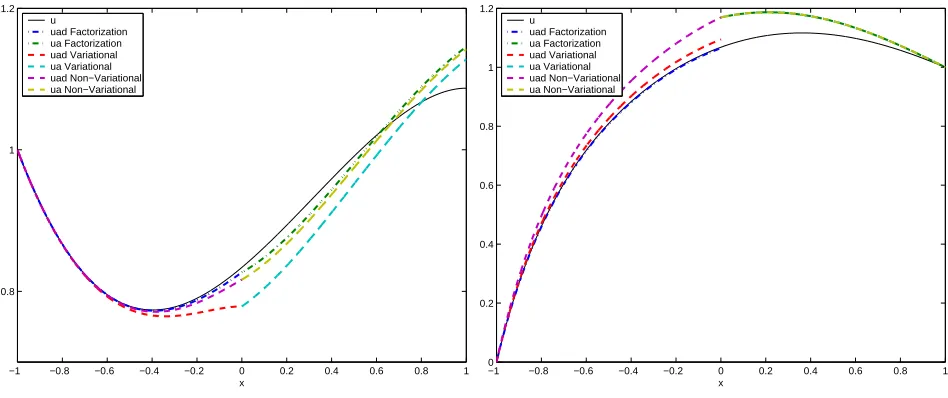
Figure 1. Approximations obtained with the various approaches, compared to the fully viscous solution, on the left for a positive advection, and on the right for a negative one.
grid points in each subregion, including boundary nodes, which leads to a discretization step h= 5.0025e−04 and ensures that solutions do not have spurious oscillations for the values ofν we use.
In the first set of experiments, we use a positive advection a = 1, ν = 1
4, with a Dirichlet condition on
the left, u(−1) = 1, and a homogeneous Neumann condition on the right u′(1) = 0. In Figure 1 we show on the left the approximations obtained with the various approaches, compared to the fully viscous solution u. Clearly the new coupling conditions lead to the best approximation in the viscous region, followed by the non-variational ones. The non-variational conditions lead to a significantly less good approximation, as we expect from our asymptotic analysis. In the inviscid region, the three approaches are comparable. Note that while the new coupling conditions lead to a non-iterative algorithm, where one simply first computes the modified advection problem, then the advection diffusion problem and finally the advection correction, both the variational and non-variational approaches are solved by an iteration per subdomain, and we chose to relax the Dirichlet variables, in the variational case by a relaxation parameter proportional toν, and in the non-variational case by a relaxation parameter proportional toν201, which turned out to lead to convergence in 7 and 8 iterations respectively.
Next we chose a negative advection, a =−1, ν = 1
4, with a homogeneous Dirichlet condition on the left,
u(−1) = 0, and an inhomogeneous Dirichlet condition on the rightu(1) = 1. In Figure 1 we show on the right the approximations obtained with the new coupling conditions, compared to the variational and non-variational approaches. Again the approximation obtained with the new coupling conditions is significantly better in the viscous region than the one obtained with the other ones, as expected from the analysis: the new approximation can hardly be distinguished in the plot from the fully viscous solution, even though in the inviscid region, the same inaccurate solution is computed. In this case, none of the algorithms requires iteration.
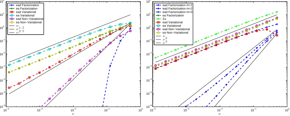
An asymptotic comparison of the error as a function ofν for ν small is shown in Figure 2, on the left for the case of positive advection, and on the right for negative advection. These numerical results show that the asymptotic analysis, summarized in Table 1 becomes relevant already for moderately smallν, and that the new coupling conditions are largely superior for the viscous approximation qualities of the solution.
5.
Conclusions
10−4 10−3 10−2 10−1 100 10−6
10−5 10−4 10−3 10−2 10−1 100 101 102
ead Factorization ea Factorization ead Variational ea Variational ead Non−Variational ea Non−Variational
ν
ν ν1
.5 ν2.5
10−4 10−3 10−2 10−1 100 10−6
10−5 10−4 10−3 10−2 10−1 100 101 102
ead Factorization m=1 ead Factorization m=2 ead Factorization m=3 ea Factorization ead Variational ea Variational ead Non−Variational ea Non−Variational
˜ea
ν
ν ν2
ν3
Figure 2. Asymptotic comparison of the error for the various coupling conditions, on the left for positive, and on the right for negative advection.
coupled solutions that are much closer to the fully viscous solution than any other coupling conditions from the literature. When a > 0, the computational cost of the new algorithm is significantly lower compared to the other coupling strategies, since no iterations are needed. For a < 0, the computational cost of the three approaches is comparable.
While the factorization approach can be generalized to higher dimensional problems and other equations, the factors will then in general contain non-local operators, which need to be approximated for convenient use as transmission conditions. In the context of coupling conditions, we will be most interested in approximations for small viscosity. As a first step into this direction, we will generalize our coupling conditions to advection reaction diffusion problems in higher dimensions.
References
[1] R. Arina and C. Canuto. A self-adaptive domain decomposition for the viscous/inviscid coupling. I. Burgers equation.Journal of Computational Physics, 105:290–300, 1993.
[2] I. P. Boglaev. The solution of a singularly perturbed convection-diffusion problem by an iterative domain decomposition method.Numerical Algorithms, 31:27–46, 2002.
[3] F. Brezzi, C. Canuto, and A. Russo. A self-adaptive formulation for the Euler-Navier Stokes coupling.Comput. Methods Appl. Mech. Eng., 73:317–330, 1989.
[4] C. A. Coclici, G. Morosanu, and W. L. Wendland. The coupling of hyperbolic and elliptic boundary value problems with variable coefficients.Mathematical Methods in the Applied Sciences, 23:401–440, 2000.
[5] C. A. Coclici, W. L. Wendland, J. Heiermann, and M. Auweter-Kurtz. A heterogeneous domain decomposition for initial-boundary value problems with conservation laws and electromagnetic fields. In T. Chan, T. Kako, H. Kawarada, and O. Piron-neau, editors,Twelfth International Conference on Domain Decomposition Methods, Chiba, Japan, pages 281–288, Bergen, 2001. Domain Decomposition Press.
[6] S. Deparis, M. Discacciati, G. Fourestey, and A. Quarteroni. Heterogeneous domain decomposition methods for fluid-structure interaction problems. In O. B. Widlund and D. E. Keyes, editors,Domain Decomposition Methods in Science and Engineering XVI, volume XVI ofLecture Notes in Computational Science and Engineering 55, pages 41–52. Springer-Verlag, 2007. [7] E. Dubach.Contribution `a la R´esolution des ´Equations fluides en domaine non born´e. PhD thesis, Universit´e Paris 13, 1993. [8] M. V. Dyke.Perturbation Methods in Fluid Dynamics. Academic Press, New York, 1964.
[10] M. Gander and F. Nataf. AILU: A preconditioner based on the analytic factorization of the elliptic operator.Numerical Linear Algebra with Applications, 7:543–567, 2000.
[11] M. J. Gander. Optimized Schwarz methods.SIAM J. Numer. Anal., 44(2):699–731, 2006.
[12] M. J. Gander, L. Halpern, C. Japhet, and V. Martin. Advection diffusion problems with pure advection approximation in subregions. In O. B. Widlund and D. E. Keyes, editors, Domain Decomposition Methods in Science and Engineering XVI, volume XVI ofLecture Notes in Computational Science and Engineering 55, pages 239–246. Springer-Verlag, 2007.
[13] M. Garbey and H. G. Kaper. Heterogeneous domain decomposition for singularly perturbed boundary problems.SIAM J. Nu-mer. Anal., 34:1513–1544, 1997.
[14] F. Gastaldi and A. Quarteroni. On the coupling of hyperbolic and parabolic systems: Analytical and numerical approach.
Applied Numerical Mathematics 6, 6:3–31, 1989.
[15] F. Gastaldi, A. Quarteroni, and G. S. Landriani. On the coupling of two dimensional hyperbolic and elliptic equations : Analytical and numerical approach. In T. C. et al eds., editor, Third International Symposium on Domain Decomposition Methods for Partial Differential Equations, pages 22–63, Philadelphia, 1990. SIAM.
[16] E. H. H. H. A. Schmatz. Zonal solutions for airfoils using Euler, boundary-layer and Navier-Stokes equations. In A. G. for Aerospace Research & Development, editor,Applications of computational fluid dynamics in aeronautics: papers presented at the Fluid Dynamics Panel Symposium in Aix-en-Provence, France, number 412, pages 20–1–20–13. AGARD conference proceedings, 1986.
[17] R. Lock and B. Williams. Viscous-inviscid interactions in external aerodynamics.Prof. Aerospace Sci., 24:51–171, 1987. [18] J. P. Loh´eac, F. Nataf, and M. Schatzman. Parabolic approximations of the convection-diffusion equation. Mathematics of
computation, 60:515–530, 1993.
[19] A. Quarteroni, F. Pasquarelli, and A. Valli. Heterogeneous domain decomposition principles, algorithms, applications. In D. E. Keyes, T. F. Chan, G. A. Meurant, J. S. Scroggs, and R. G. Voigt, editors, Fifth International Symposium on Domain Decomposition Methods for Partial Differential Equations, pages 129–150, Philadelphia, PA, 1992. SIAM.
[20] A. Quarteroni and L. Stolcis. Homogeneous and heterogeneous domain decomposition for compressible fluid flows at high Reynolds numbers.Numerical Methods for Fluid Dynamics, 5:113–128, 1995.