An algorithm for the anchor points of the PPS of the CCR model

(1)

Int. J. Data Envelopment Analysis (ISSN 2345-458X) Vol.5, No.4, Year 2017 Article ID IJDEA-00422, 14 pages

Research Article

An Algorithm for the Anchor Points of the

PPS of the CCR Model

D. Akbarian*

Department of Mathematics, Arak Branch, Islamic Azad University, Arak, Iran.

Received 20 May 2017, Accepted 28 September 2017 Abstract

Anchor DMUs are a new class in the general classification of Decision Making Units (DMUs) in Data Envelopment Analysis (DEA). An anchor DMU in DEA is an extreme-efficient DMU that defines the transition from the efficient frontier to the free-disposability part of the boundary of the Production Possibility Set (PPS). In this paper, the anchor points of the PPS of the CCR model are investigated. A basic definition of anchor point based on the supporting hyperplanes of the PPS of CCR model is provided. Then, by using a variant of super-efficiency models, the necessary and sufficient conditions for a DMU to be an anchor DMU are provided via some theorems. To illustrate the applicability of the proposed model, some numerical examples are finally given.

Keywords: Data Envelopment Analysis (DEA); Production Possibility Set (PPS), Efficient and inefficient frontier.

*. Email: d [email protected], [email protected]

(2)

1. Introduction

An anchor point in DEA is an extreme-efficient DMU lying on the intersection of some strongly and weakly efficient frontiers of the PPS. An anchor point is, therefore, an extreme-efficient DMU in which some inputs can increase and/or some outputs can decrease without passing through the interior of the PPS. Anchor points play a significant role in DEA theory and applications. The concept of anchor point was used in Thanassoulis and Allen [11] (1998) for the generation of unobserved DMUs in order to reduce appropriately the DEA-inefficient boundary of the PPS. Anchor points were first named and identified by Allen and Thanassoulis [2] (2004). They proposed a method for detecting anchor points of the constant returns to scale production possibility set (CRS-PPS) with one input and multiple outputs. However, their method is not applicable to multiple inputs and outputs. Thanassoulis et al. [11](2012) proposed another approach to identify anchor points, using the radial efficiency scores and slack variables at the optimal solution of envelopment models. They extended the proposed approach in Allen and Thanassoulis [12] (2004) to the multiple inputs and outputs case in variable returns to scale production possibility set (VRS-PPS) in order to improve envelopment by means of unobserved DMUs. Bougnol and Dulá [3] (2009) defined the anchor point for the VRS-PPS. They provided a specialized procedure to identify anchor points based on their geometrical properties. Rouse [10](2004) employed this idea in identifying prices for health care services. For more detail about the notion and applications of the anchor DMUs, see Bougnol [4] (2001) and Allen and Thanassoulis [2] (2004). Since the set of anchor DMUs is a subset of the set of extreme DMUs, the set of extreme DMUs must be obtained. For this aim, one can use the proposed algorithms in Charnes,

Cooper and Thrall [6] (1991) as well as Dulá and López [7] (2006) among others. This paper provides a definition for the anchor point of the CRS-PPS. Subsequently, it utilizes a novel approach to identify the anchor points of the PPS of the CCR model in the multiple inputs and outputs case; through testing all CCR-efficient DMUs by a variant of super-efficiency models (see models (3) and (4), after eliminating the inefficient-CCR DMUs from the PPS). In fact, extreme and non-extreme CCR-efficient DMUs and anchor DMUs can be obtained, using models (3) and (4). An advantage of the proposed approach is in determining which inputs (outputs) of anchor DMUs can increase (decrease) without penetrating into the interior of the production possibility set. Another advantage of the proposed approach is in discovering the edges of the PPS on which the anchor DMUs lie; whereas the aforementioned methods are unable to do these two advantages. Some useful facts related to the properties of models (3) and (4) and the necessary and sufficient conditions for a DMU to be an anchor DMU are stated and proved. In addition, three numerical examples are provided. 2. Background

Consider a set of n DMUs which is associated with m inputs and s outputs.

Particularly, each DM

( ; ) ( {1, , }) j j j

U  X Y j  J n

consumes amount xij (> 0) of inputi and produces amount yrj (> 0) of output r. The production possibility set T,





(3)

1413 et al. [5] (1978)):



,



_j _j, _j _j, _j 0,

j J j J

T X Y X X Y Y  j J

              





in which Xj and Yj are vectors of inputs and outputs of DMU_j, respectively.

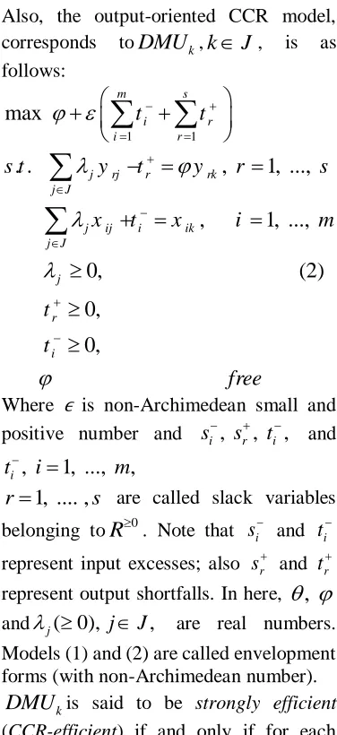
We will employ a DMU classification based on the categories (i) CCR-inefficient (weak efficient and interior), (ii) non-extreme CCR-efficient, and (iii) non-extreme CCR-efficient. The three categories define the subsets `F ', `E', and `E ', respectively. These three subsets partition the set J. Any DMU in E; lies on the boundary (non-extreme) ray and any DMU in E; lies on the extreme ray of the PPS of the CCR model and named as extreme DMU. The set E*_{is also called the}_frame_of_J_{. The} frames are important in DEA because the PPS of the DEA models are constructed by them and the exclusion each of them alters the shape of the PPS. The PPS of the CCR model is depicted in Figures (1) and (2). In Figure (1),



1, 2, 3, 4



J  D D D D , F 

 

D₄ , E

 

D₃

and *





1, 2

E  D D . Also D1 and D2 are anchor DMUs.

The input-oriented CCR model, corresponds to

DMU

_k,kJ, is given by:

1 1

min

. .

,

1, ...,

,

1, ...,

0, (1)

0,

m s i r i r

j rj r rk j J

j ij i ik j J

j r i

s

s t

y

s

y

r

s

x

s

x

i

m

s

 









         

















 



 







free

Also, the output-oriented CCR model, corresponds to

DMU

_k,kJ , is as follows:

1 1

max

. .

,

1, ...,

,

1, ...,

0,

(2)

0,

m s i r i r

j rj r rk j J

j ij i ik j J

j r i

t

s t

y

t

y

r

s

x

t

x

i

m

t

 









         

















 



 







free

Where ϵ is non-Archimedean small and positive number and

s

_i

, , ,

s

_r

t

_i and

, 1, ..., ,

i

t i m

1, .... ,

r s are called slack variables belonging to

R

0. Note that

s

i



and

t

i



represent input excesses; also s_r and t_r

represent output shortfalls. In here,

 

,

and



j( 0),  jJ, are real numbers.

Models (1) and (2) are called envelopment forms (with non-Archimedean number).

k

DMU

is said to be strongly efficient (CCR-efficient) if and only if for each optimal solutions, either (i) or (ii) happen: (i)



* 1 and * *

(

s

,

s

)

(0, 0)

(ii)



* 1 and * *

(

t

,

t

)

(0, 0)

k

DMU

is said to be weak efficient if and only if for some optimal solutions, either (v) or (iv) happen:

(v)



* 1 and * *

(

s

 ,

s

 )

(0, 0)

(iv)



*1 and * *

(

t

 ,

t

)

(0, 0)

(4)

Each inefficient and weak efficient DMU in the CCR model is said to be a CCR-inefficient DMU.

Efficient Frontier is the set of all points (real or virtual DMUs) with efficiency score is equal to unity. Efficient frontier is divided into two categories:

i) Strong efficient frontier is the set of all (real or virtual) strong efficient (CCR efficient) DMUs.

ii) Weak efficient frontier in which all its relative interior points (real or virtual DMUs) are weak efficient DMUs.

DM Uk = (Xk, Yk) is said to be non-dominated if and only if there is not any DMU = (X, Y) (real or virtual) such that:

(X Y_k, ) (_k  X Y, ) and (X Yk, k) ( X Y, ) We use the following theorem in the next section.

Theorem 1: There does not exist any virtual DMU (a member of the PPS) that dominates an

DEA-efficient DMU.

Proof. See H. Fukuyama et al. (2012). In this paper, corresponding to each strong

efficient DMU

, the virtual

DMUs l



₁ ,..., ,..., , ₁,...,



j j lj mj j sj

DMU  x x  x y y

and q



₁ ,..., , ₁ ,... ,...,



j j mj j qj sj

DMU  x x y y  y

in which

 

, 0, are called “Dominated Input Virtual" DIVkland “Dominated Output Virtual" q

k

DOV DMUs,

respectively. These virtual DMUs are either interior points of the PPS of the CCR model or lie on the some weak efficient frontiers (see theorems 3 and 6 and the proof of theorem 4). In the latter case we call these virtual DMUs as “weak efficient virtual DMUs" or WEV DMUs, hereafter. It is important to note that the WEV DMUs play an important role in identifying anchor points. Accordingly, this paper tries to find them. In figure 1, DMU





1 12

,

22

,

12

D



x

y

is strong efficient DMU andDIV₁2,

D

₁

 



x

₁₂

,

x

₂₂

+ ,



y

₁₂



is a WEV DMU. In addition, in figure 2, 2

1 1

DOV D andDOV D11 1,

corresponding to DMU D1, are WEV DMUs.

The following definition introduces the anchor points of the PPS of the CCR model.

Figure 1: DIV21 DMU D2 is a WEV DMU and also model 3 corresponding to D2with l=1 is

infeasible therefore, D₂ is an anchor point. 2

1. (*) is used for optimal solution

1 1

( ,..., , ,..., )

j j mj j sj

(5)

1415

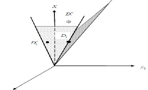
Figure 2: Model 4 corresponding to DMU

D

₁ with q = 2 is infeasible therefore, D1 is an anchor point. Also, DIV D₁1 ₁ is an interior point 7.

Definition. DMU_kE*is an anchor DMU if it belongs to an unbounded face of the PPS of the CCR model.

Remark1. By the above definition; *

k

DMU E is an anchor DMU if there

exist some l (or q) so thatDIV_kl (or q

k

DOV ) DMUs are WEV DMUs.

In figure 1, DIV21 DMU D2' is a WEV DMU and so, D₂' is an anchor point. Throughout this paper, we must assume that there are not any two strong efficient DMUs as ( , )x y and ( , )tx ty for allt > 0 and

t



1

. Otherwise, one of them must be deleted.

3. Identifying the anchor DMUs of the PPS of the CCR model

In this section, the anchor DMUs of the PPS of the CCR model are defined in the following way.

First, eachDMU_k;



kJ



, is evaluated by models (1) or (2). Then, we hold all CCR-efficient

DMUs, and remove other DMUs. Suppose that the set of all CCR-efficient DMUs is denoted by

E



(

 

E

*

)

. Corresponding

to each



1

,...,

,

1

,...,



, (

')

k k mk k sk

DMU



x

y

k



E

, the following models are solved:

  '

min

. . ,

1, ..., k

l

k

j rj rk j E k

s t y y

r s



  







 

'

,

1, ..., ,

,

0,

'

1, ...,

k j ij ik j E k

k k

j lj l lk j E k

k j k l

x

i

m i

l

x

j E

k

free l

m









 











 





(3)

 

  '

'

max

. . ,

1, ..., ,

,

1, ..., ,

k q

k

j rj rk j E k

k k

j qj q qk j E k

k

j ij ik j E k

s t y y

r s r q

y y

x x

i m









 



 









(6)

 

0, '

1, ...,

k j k q

j E k

free q s





  



The following Theorems are held for models (3) and (4). The theorems 3-8 provide the necessary and sufficient conditions for a DMU to be an anchor DMU.

Theorem 2: In model (3) (or (4)), if for somel(or q),



_lk*1 (or

,

k*

1

q





) or if for some l (or q), model (3) (or model (4))

is infeasible, then,

k

DMU is an extreme DMU and vice versa.

Proof. Suppose that *

1

k l



 . First, we show that

DMU

_k is CCR-efficient. By contradiction, suppose that

DMU

_kis CCR-inefficient. Let * * *

( ,

s s

,  ) be the optimal solution of model (1).

Two cases can occur: (i)



*1_and * *

(

s

,

s

)(0, 0)

(ii)



*1

in each case it can be shown that k* 1

l



 , a contradiction.

Now we show that

DMU

_k is, in fact, an extreme CCR-efficient DMU. By contradiction suppose that

DMU

_k is a non-extreme CCR-efficient. So, the following system has solution:

'

,

0,

'

j j k

j E

j j k

j E j

y

x

j

E



 









(5)

Suppose that



j, jE' is a solution of

the above system. If



k



0

then,

( k 1, , -{ })

j

l j j E k











 is a solution of model (3). Therefore,



_lk* 1, a

contradiction. On the other hand if



k



0

system (5) can be rewritten as follows:

' { }

(1

)

,

(1

)

j _j k _k

j E k

j _j k _k

j E k

y

x



   

 



By dividing both sides of the above equations by (1





k



0

); a solution of model (3) is obtained as

1, , '-{ }

1

(

k j

)

l j

j

j E k 

 



  

 .

Therefore,



lk*1, a contradiction. Thus,

k

DMU

is an extreme CCR-efficient DMU. Now, suppose that for some l, model (3) is infeasible. In the similar manner, it can be shown that DMUk is an extreme CCR-efficient DMU. Conversely, suppose that

DMU

_kis extreme DMU and model (3) is feasible. We show that k* 1

l





. Consider the following problem corresponding to

DMU

_k:

'

min

. . ,

1, ...,

,

1, ..., ,

k l

k

j rj r rk

j E k

j ij i ik

j E

s t y s y

r s

x s x

i m i l





          



(6) ' ' ' , 0, '

, 0, 1, ..., 1, ..., , 1, ...,

k k

j lj l l lk j E k j r i k l

x s x

j E

s s r s i m

free l m

               



Now suppose that *_{( 1),} ' *k l

   and



lk* are the optimal objective functions of the models (1), (6) and (3) with respect to

k

(7)

1417 show that



*



_l' *k 



_lk* Therefore,

*

1

k l



 . This completes the proof. Corollary:In models (3) and (4), for each land q k* k* 1

l q







 if and only ifDM Uk is a non-extreme CCR-efficient DMU.

Proof. Omitted.

Theorem 3: In a single input case,

corresponding to each



1

,

1

,...,



k k k sk

DMU



x

y

the DIVk1





'

1

,

1

,...,

k k k sk

DMU



x





y

in which

0





, is an interior point of the PPS of the CCR model.

Proof. First, we add DMU_k' to the PPS and then, evaluate its performance by the input and output-oriented CCR models (see models (1) and (2)). It is enough to show that



*1_and



* 1. Consider the input-oriented CCR model corresponding to virtual DMU

DMU

_k



as follows:

'

1 1 1

'

min

. . , 1, ..., ( ) ( ), 0, '

j rj k rk rk j E

j j k k k

j E j

s t y y y r s

x x x

j E free                     



(7) 1 1

0 ( ), 1, 0, k ( 1)

j k _k

k x j k x               _   

is a feasible solution of (7). Since model (7) has a minimization-type objective function,



*1; where “*” is used to

indicate optimality. In a similar manner, it can be shown that in output-oriented maximization problem,



*1 Therefore,

k

DMU

is an interior point of the PPS. This completes the proof.

In Figure 2, corresponding to DMU





1 11, 11, 21

D  x y y , the





1 ''

1 1 11 , 11, 21

DIV D  x  y y is an interior point of the PPS.

Theorem 4: In a multiple inputs case, if for some l, model (3) is infeasible, then extreme

CCR-efficient

DMU

_k is an anchor DMU.

Proof. In view of Remark 1, we show that if for some l, model (3) is infeasible, then, the DIVkl

1 ( 1) ( 1) 1

,..., , ,

,... , , ,...,

j l j lj k

l j mj j sj

x x x

DMU

x x y y

        _ _   0



 ,

is a WEV DMU. For this aim, it can be shown that in the performance evaluation of

DMU

_k



, using model (2);



*1. Consider model (2); corresponding to virtual DMU

DMU

_k



as follows (without

ϵ): ' ' ' max . . ,

1, ...,

,

1, ..., ,

( ) ,

0, ' 0,

j rj k rk rk j E

j ij k ik ik j E

j lj k lk lk j E

j k

s t y y y

r s

x x x

i m i l

x x x

j E                             



 free (8)

By contradiction, suppose that

* *

( '), , ( 1)

(

j jE  k 

)

is the optimal

(8)











 



* * * ' { } * * * ' { } * * * ' { } 1 ,

1, ...,

1 ,

1, ..., ,

1 1 ,

j rj k k rk j E k

j ij k k ik j E k

j lj k k lk k j E k

y y

r s

x x

i m i l

x x                               



(9)

From model (9), it is easy to show that

* *

1



k 



k 0. Divide both sides of

model (9) by 1



k* 



k* 0 and define

* * * *, ' { } 1 j j k k

j E k 



 

  

  ; so, model

(9) becomes as follows:

' { }

,

1, ...,

,

1, ..., ,

j rj rk

j E k

j ij ik j E k

j lj lk j E k

y

r

s

x

i

m i

l

x





     

















(10)

in which *

* * 1 1 k k k           _ _   

. Since



0, there is



ˆ 0



; so that x_lk   ˆx_lk; therefore, the constraints of model (10) can be rewritten as follows:

' { }

, 1, ..., , 1, ..., , ˆ

j rj rk j E k

j ij ik j E k

j lj lk j E k

y y r s

x x i m i l

x x





           



So,



_j



j E' { } , k



ˆ



is a feasible solution for model (3); a contradiction. This implies that



* 1 i.e.

DMU

_k



lies on the efficient frontier. Now, since

k

DMU



is dominated by CCR-efficient k

DMU

, so, the DIVkl DMU_k' is a WEV

DMU. Therefore, in view of Remark 1 k

DMU

is an anchor DMU. This completes the proof.

In Figure 1, model (3) corresponding to DMU

D

₂



(

x

₁₂

,

x

₂₂

,

y

₁₂

)

, with l = 1, is infeasible; so, DMU D2 is an anchor DMU. The following theorem is, in fact, the converse of Theorem 4.

Theorem 5: In multiple inputs case, if extreme CCR-efficiency DMU



1

, ...,

, y , ..., y

1



k k lk mk k sk

DMU



x

is an anchor DMU and theDIV_k1 DMU is a WEV DMU; then model (3) is infeasible.

Proof. By contradiction, suppose that model (3) is feasible. The first constraint of the model (3) implies that the optimal solution of model (3) is bounded. Suppose that, * *

, ( )

(

k

)

l j j k





is an optimal solution of it. Note that the first constraint of model (3) is tight at optimality.

We first show that *

1

k l



 . By

contradiction suppose *

1

k l



 . If *

1 k l



 we have: * ' { } * ' { } * ' { } ,

1, ..., , , 1, ...,

k

j lj l lk lk j E k

k

j ij ik j E k

k

j rj rk j E k

x x x

x x

i m i l

y y r s                 



(11)

(9)

1419 * 1 ' { } * ' { } * ' { } * 1 ' { } * ' { } , ..., , ..., , , ..., k j j j E k

k j lj j E k

k j mj j E k

k j j j E k

k j sj j E k

x x x y y



                                     



Dominates the CCR-efficient

DMU

_k, a contradiction (see Theorem 1). Now, if

*

1 k l



 , we have:

* ' { } * ' { } * ' { }

,

1, ..., ,

,

1, ...,

k

j lj lk j E k

k

j ij ik j E k

k

j rj rk j E k

x

i

m i

l

y

r

s



     















(12)

At least one of the inequality constraints of (12) is a strict inequality, because, otherwise, the CCR-efficient

DMU

_k, is not extreme DMU and so *

1

k l



 .

Therefore, there exist 0 so that *

lkxlk xlk



 



. This means that, the

virtual DMU

1 ( 1)

( 1) 1

, ..., , , ,..., , y , ..., y

k l k lk k

l k mk k sk

x x x

DMU x x



       _ _  

is, in fact, an observed DMU belongs to the PPS of the CCR model. This is a contradiction because; the CCR-inefficient DMUs had been eliminated from the PPS of the CCR model. The proof is completed. Theorem 6: In a single output case, for each

DMU

_k





x

₁_k

,...,

x

_mk

, y

₁_k



the

1

k

DOV

DMU

_k





x

₁_k

,...,

x

_mk

, y

₁_k







in which





0

is an interior point of the PPS of the CCR model.

Proof. The proof is similar to the theorem 3 and so, the details are omitted.

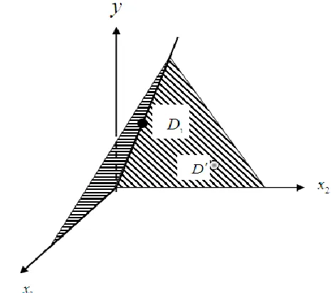
In Figure 3, 1

1

DOV DMU



11 12 11



' , x , y

D  x  , corresponding to DMU

D

₁





x

₁₁

, x , y

₁₂ ₁₁



is an interior point of the PPS.

Theorem 7:In multiple outputs case, if for someq, model (4) is infeasible, then, CCR-efficient DMU_kis an anchor DMU.

Proof. The proof is similar to theorem 4 except that it can be shown that in the performance evaluation of DMU_k using model (1); *

1



 .

In Figure 2, model (4) corresponding to DMUD₁ 



x₁₁, y , y₁₁ ₂₁



, with q = 2, is infeasible, so, the DOV12 DMU is a





1 11

, y , y

11 21

D

 

x





WEV DMU

(10)

Figure 3: Theorem 6. DOV D11 is interior point of the PPS.

Theorem 8: In multiple outputs case, let extreme CCR-efficiency DMU



1 , ..., , y , ..., y ,..., y1



k k mk k qk sk

DMU  x x

is an anchor DMU and the DOVkq DMU is a WEV DMU; then model (4) is infeasible.

Proof. The proof is similar to the theorem 5 except that by contradiction it must be assumed that the model (4) is feasible. So, we omit it.

Now, by theorem 2; all extreme DMUs of the PPS of the CCR model can be found. Also, by theorems 4 and 5; all anchor DMUs for which the DIV_kl DMUs

1 ( 1)

( 1) 1

, ...,

,

...,

, y , ..., y

k l k lk k

l k mk k sk

x

DMU

x











  









are WEV DMUs can be found and by theorems 7 and 8; all anchor DMUs for

which the DOV_kq DMUs



1 , ..., , y , ..., y1 ,..., y



k k mk k qk sk

DMU  x x 



are WEV DMUs can be found and therefore, all anchor points of the PPS of the CCR model can be found.

Now we are in the position to put all together the ingredients of the method. Summary of finding all anchor DMUs algorithm

 Step 1. Evaluate n DMUs with a suitable form of models (1) and, (2). Hold all CCR-efficient DMUs and remove other DMUs. Put indices of these CCR-efficient DMUs in E′.

 Step 2. Evaluate each DMU in E′ with models (3) and (4). (Note that in the single input case we don't use model (3) and in the single output case we don't use model (4)).

 Step 3. If for some l (or q) the model (3) (or (4)) is infeasible, then,

DMU

_kis an anchor DMU andDIV_kl (orDOV_kq)

k

DMU



is WEV DMU.

 Step 4. If each DMU in E′ are evaluated by models (3) and (4), stop. Otherwise, go to step 1.

(11)

1421

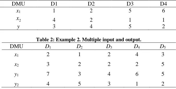
DMU D1 D2 D3 D4

x1 1 2 5 6

2

x ₄ ₂ ₁ ₁

y 3 4 5 2

Table 2: Example 2. Multiple input and output.

DMU D1 D2 D3 D4 D5

x1 2 1 2 4 3

x2 3 2 2 2 5

y1 7 3 4 6 5

y2 4 5 3 1 2

4. Numerical Examples Example 1(Single output case)

Table 1 shows data for 4 DMUs with two inputs and one output. Using the CCR model (1), CCR-efficient DMUs are determined to be

D

₁, D₂ andD₃. So,



1, 2, 3



E

 

. Remove CCR-inefficient DMU D3 from PPS and solve model (3) corresponding to CCR-efficient DMUs

D

₁

, D2and D3.

The following results are yielded:

By theorem 2, DMUs

D

₁, D2 andD3lie on the extreme rays of the PPS. Model (3) corresponding to DMU

D

₁ with l = 2 and DMU D3 with l = 1 is infeasible. So, by theorem 4 DMUs

D

₁and D3 are anchor DMUs and DIV₁2 and DIV₃l DMUs are WEV DMUs. Note that model (3) corresponding to DMU D2with l = 1, 2 is feasible. So, by theorem 5, DMU D2 is not anchor DMU.

Example 2 (Multiple outputs and inputs case)

Table 2 shows data for 5 DMUs with two inputs and two outputs. Running model

(1) (or (2)) shows that

D

₁, D₂ andD₄ are efficient and other DMUs are CCR-inefficient. So,

E

 



1, 2, 4



. By applying models (3) and (4) to each

DMU

_k,

kEthe results reported in table 3 are obtained. In table 3, “INFES" and “FES” denotes “infeasible” and “feasible”, respectively. For instance, “INFES” in the first row and the second column means that model (3), corresponding to DMU

D

₁

with l=2, is infeasible. So, by theorem 4, 1

D

is an anchor DMU and DIV₁2 DMU 1 (2, 3 + , 7, 4)

D 



is a WEV DMU.

Using theorems 4 and 7 and the information of table 3, all

DMU

_k, kE

are anchor DMUs.

Example 3(Real word data)

We evaluated the data of 20 branches of a bank in Iran using the proposed method. The data was previously analyzed by Amirteimoori et al. (2005), (see table (4)). Running the DEA model (1) (or (2)) resulted in

E = 1, 4, 7,12,15,17, 20







. Using the proposed method, all DMUs in

E



are found to be anchor DMUs. Also 1,2

1

DIV , DIV41,2,3, DIV71,2,3, DIV122, 1,2,3

15

DIV , DIV171,2,3,

2,3 20

(12)

1,2 4

DOV , DOV₇1,3, DOV₁₂1,3 , DOV₁₅2,3, 1,3

17

DOV , DOV₂₀1,2 DMUs are WEV DMUs. For instance, DIV₁₅1,2,3means that,

15

DMU is an anchor point and the first, second and the third inputs of

15

DMU can be increased without penetrating the interior of the PPS. Also,

1,3 7

DOV means that,

DMU

₇is an anchor point and the first and third outputs of

7

DMU

can decrease without penetrating the interior of the PPS.

Table 3: Example 2. The results of evaluation CCR-efficient DMUs by models (3) and (4).

DMU l q

1 2 1 2

D1 FES INFES FES INFES

D2 INFES INFES INFES FES

D4 INFES FES FES INFES

Table 4: Example 3. DMUs' data (extracted from [Amirteimoori et al. (2005), p. 689]).

input output

Branch Staﬀ Computer terminals Space m2 Deposits Loans Charge

1 0.9503 0.70 0.1550 0.1900 0.5214 0.2926

2 0.7962 0.60 1.0000 0.2266 0.6274 0.4624

3 0.7982 0.75 0.5125 0.2283 0.9703 0.2606

4 0.8651 0.55 0.2100 0.1927 0.6324 1.0000

5 0.8151 0.85 0.2675 0.2333 0.7221 0.2463

6 0.8416 0.65 0.5000 0.2069 0.6025 0.5689

7 0.7189 0.60 0.3500 0.1824 0.9000 0.7158

8 0.7853 0.75 0.1200 0.1250 0.2340 0.2977

9 0.4756 0.60 0.1350 0.0801 0.3643 0.2439

10 0.6782 0.55 0.5100 0.0818 0.1835 0.0486

11 0.7112 1.00 0.3050 0.2117 0.3179 0.4031

12 0.8113 0.65 0.2550 0.1227 0.9225 0.6279

13 0.6586 0.85 0.3400 0.1755 0.6452 0.2605

14 0.9763 0.80 0.5400 0.1443 0.5143 0.2433

15 0.6845 0.95 0.4500 1.0000 0.2617 0.0982

16 0.6127 0.90 0.5250 0.1151 0.4021 0.4641

17 1.0000 0.60 0.2050 0.0900 1.0000 0.1614

18 0.6337 0.65 0.2350 0.0591 0.3492 0.0678

19 0.3715 0.70 0.2375 0.0385 0.1898 0.1112

20 0.5827 0.55 0.5000 0.1101 0.6145 0.7643

5. Conclusions

Anchor points play an important role in DEA theory and application. They delineate the efficient frontier from the free-disposability portion of the PPS frontier. Their identification has several notable DEA applications such as the construction of \unobserved" DMUs in order to reduce appropriately the

(13)

(14)

References

[1] Amirteimoori A., Kordrostami S., (2005). Efficient surfaces and an efficiency index in DEA: a constant returns to scale, Applied Mathematics and Computation, 163 683-691.

[2] Allen, R., & Thanassoulis, E. (2004). Improving envelopment in data envelopment analysis. European Journal of Operational Research, 154, 363-379. [3] Bougnol M-L., Dula , J.H., (2009). \Anchor points in DEA", European Journal of Operational Research, 192 668-676.

[4] Bougnol, M. L. (2001). Nonparametric frontier analysis with multiple constituencies. Ph.D. dissertation, The University of Mississippi.

[5] Charnes A., Cooper W.W., Rhodes E., (1978). \Measuring the efficiency of decision making units", European Journal of Operational Research, 2 (6) 429-444. [6] Charnes, A., Cooper, W. W., & Thrall, R. M. (1991). A structure for classifying and characterizing efficiency and inefficiency in data envelopment analysis. Journal of Productivity Analysis 2 197-237.

[7] Dula, J. H., & Lopez, F. J. (2006). Algorithms for the frame of a nitely generated unbounded polyhedron. INFORMS Journal on Computing 18 97-110.

[8] Fukuyama H., Mirdehghan S.M., (2012). Identifying the efficiency status in network DEA".European Journal of Operational Research 220 85-92.

[9] Jahanshahloo G.R., Hosseinzadeh Lot F., Akbarian D., (2010). Finding weak defining hyperplanes of PPS of the BCC model". Applied Mathematical Modeling, 34 3321-3332

[10] Rouse P., (2004). Using DEA to set prices for health care delivery in New Zealand hospitals, Working paper. The University of Auckland, New Zealand. [11] Thanassoulis E., Allen R., (1998). Simulating weights restrictions in data envelopment analysis by means of unobserved DMUs". Management Science 44 (4) 586-594.

[12] Thanassoulis E., Kortelainen M., & Allen R., (2012). \Improving envelopment in data envelopment analysis under variable returns to scale.". European Journal of Operational Research 218 175-185.