Improving Accuracy in Earthwork Volume Estimation for Proposed Forest Roads Using a High-Resolution Digital Elevation Model
18
0
0
Full text
(2) M. Contreras et al.. Improving Accuracy in Earthwork Volume Estimation for Proposed Forest Roads ... (125–142). Hickerson 1964 for more details). The Pappus-based method provides accurate estimates only when the two cross-sections are also of the same type (either cut or fill). Easa (1992b) also developed a mathematical method based on triple integration that can deal with transition road segments where one of two consecutive cross-sections has both cut and fill areas, while the other has only either one. This method is complicated and applicable only for road segments where the ground profile is linear (Aruga et al. 2005). These existing earthwork volume estimating methods assume that the ground slope at each road cross-section is constant, which is unlike for most hilly and mountainous terrains. Kim and Schonfeld (2001) developed two methods to estimate cross-section areas more precisely. These methods use an interpolation method (inverse distance-weighted) to obtain elevation data, and vector and parametric representation of cross-sections to account for irregular ground slopes. The accuracy of all aforementioned methods seems to improve as the distance between consecutive cross-sections decreases (Kim and Schonfeld 2001). However, cross-sections can only be derived at survey stations, and an assumption about the homogeneity of ground slopes between consecutive cross-sections has to be made. High-resolution DEMs derived from the light detection and ranging (LiDAR) technology have recently been incorporated into forest road planning and design to increase accuracy in volume estimation by using the elevation data of each raster grid cell. LiDAR technology is known to provide accurate estimates of ground surface elevation even under a dense canopy cover (Reutebuch et al. 2003). Coulter et al. (2001) applied a 1-meter resolution LiDAR-derived DEM to estimate earthwork volumes for a proposed forest road. In this method, road elevation was assigned to each grid cell within the road template to estimate earthwork volume from the difference between road and ground surface elevations. However, this simplistic method is only applicable to straight road segments. Aruga et al. (2005) developed a computer program for forest road design that also uses a 1-meter resolution DEM. Their model precisely generates cross-sections and calculates areas, and accurately estimates earthwork volumes. As the actual ground profile can be represented more accurately when a shorter distance between cross-sections is applied (Aruga et al. 2005), earthwork volume estimations using a 1-meter resolution DEM were considered »exact« and comparable with other estimates obtained from different cross-section spacings and different estimation methods. The study was focused on the optimization of road design, and, however, limited emphasis was. 126. put on numerical procedures and the study does not provide a thorough analysis of the effects of cross-section spacing on earthwork volume estimation. Although the accuracy of earthwork volume estimates is expected to increase with decreasing spacing between consecutive cross-sections, to our knowledge, there are no studies evaluating and quantifying the differences in earthwork volume estimates in various terrain conditions. In this study, we developed a computerized model to accurately estimate earthwork volumes for the proposed forest roads using a high-resolution LiDAR-derived DEM. We examined the effects of cross-section spacings on the accuracy of earthwork volume estimation by applying the model to the proposed roads in various areas under different terrain conditions and estimating earthwork volumes of the roads at different cross-section spacings. Similar to Aruga et al. (2005), we assumed that 1-meter cross-section spacing provided the »true« earthwork value in our study. Our computerized model was applied to three hypothetical forest roads laid out on low, moderate, and steep slope areas, and the earthwork volume estimates from the model were compared with those from the traditional end-area method, which considers only the cross-sections located at survey stations. Lastly, comparisons were also made on road sections with three levels of terrain ruggedness.. 2. Computerized model – Ra~unalni model The computerized model developed in this study was designed to accurately estimate cut and fill volumes for a proposed forest road using a high-resolution DEM. The main input data for the model include: i) an ASCII text file representing the LiDAR-derived DEM for the area of interest, and ii) a text file representing the x- and y-coordinates of sequential survey station points along a proposed road. Based on the cell size (1 meter in our applications) and the x-and y-coordinates of the lower left corner of DEM, the model calculates x- and y-coordinates of each grid cell in the DEM. These coordinates are used to obtain the ground elevation of each survey station point along the proposed road gradeline.. 2.1 Estimating ground elevation – Procjena visine terena Starting from the beginning-of-project (BOP), ground elevations for each survey station point (SP) are obtained from the LiDAR-derived DEM. As DEM elevation values represent the elevation at the center of the grid cell and since a given SP might not coCroat. j. for. eng. 33(2012)1.
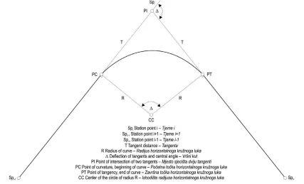
(3) Improving Accuracy in Earthwork Volume Estimation for Proposed Forest Roads ... (125–142). M. Contreras et al.. Fig. 1), and the other three adjacent cells (grid cells with a square in Fig. 1). The horizontal distances from the SP to the four grid cells are computed and their z-coordinates are obtained. The SP z-coordinate is then obtained based on the inverse distance to each adjacent grid cell and their respective elevation values (Eq. 1). Ni. Ni. j =1. j =1. SPZi = å ( dj-1 × z j ) / å dj-1. Fig. 1 Estimating ground elevation on a given point (dot) using the interpolation method based on four grid cells including the grid cell containing the point (grid cell with a cross) and three adjacent grid cells (grid cells with squares) Slika 1. Procjena visine terena odre|enoga polo`aja (to~ka) primjenom metode interpolacije zasnovane na ~etirima podacima pravilne mre`e to~aka (polje s kri`i}em) i na trima susjednim poljima (polja s kvadrati}em) incide with a grid cell center, an interpolation method is used to estimate the SP z-coordinate. The interpolation method uses inverse distance-weighted based on its four adjacent grid cells. For a given SP, (dot in Fig. 1) the model identifies the grid cell containing it (grid cell with a cross in. "j Î N i. (1). where, SPZi is the z-coordinate of the ith SP, dj is the horizontal distance from the jth grid cell to SP, zj is the z-coordinate of the jth grid cell, and Ni indicates the set of four closest grid cells to the ith SP. Once the three-dimensional coordinates of all SP are determined, the model locates a curve for each intersection point and identifies the position of the beginning and end of curve.. 2.2 Locating horizontal curves – Odre|ivanje glavnih to~aka horizontalnoga kru`noga luka We assumed all SP (n) along a proposed road except BOP and end-of-project (EOP) become intersection points (PI in Fig. 2), where curves are located to avoid sharp turns. Each horizontal curve location is determined based on the x- and y-coordinates of the SPi, (same as the PI), SPi-1 and SPi+1, and a user defined minimum allowable radius of the curve (R). In the United States, R ranges from 18 m to 40 m. Fig. 2 An example of horizontal curve design and nomenclature Slika 2. Primjer oblikovanja i osnovne sastavnice horizontalnoga kru`noga luka Croat. j. for. eng. 33(2012)1. 127.
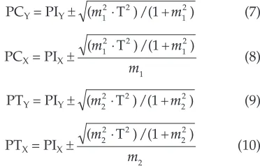
(4) M. Contreras et al.. Improving Accuracy in Earthwork Volume Estimation for Proposed Forest Roads ... (125–142). depending on the road standard (Akay 2003). Fig. 2 shows the nomenclature used in the model to determine the location of the beginning and end of the curve (PC and PT, respectively), and the location of the curve center (CC in Fig. 2), whose arc passes through PC, and PT is also determined for posterior calculations of the curve design. For each PI, represented by SPi, the model calculates the direction of the two tangent lines in a two-dimensional (x, y) Cartesian coordinate system as follows: m1 =. m2 =. diff _ y 1 diff _ x 1 diff _ y 2 diff _ x 2. =. =. yi - yi-1 xi - xi-1 yi+ 1 - yi xi+ 1 - xi. (2). PCX = PIX ±. where, Azim and m are azimuth and direction of a tangent line, respectively. Then, the central angle (D in Fig. 2) is calculated as follows: ì 360- |Azim2 - Azim1 | if |Azim2 - Azim1 |> 180 D=í (5) otherwise î |Azim2 - Azim1 | Once the angle D is obtained, the model calculates the tangent distance (T in Fig. 2) from PI to PC and PT (Eq. 6). (6). (m12 × T 2 ) /(1 + m12 ) m1. PTY = PIY ± (m22 × T 2 ) /(1 + m22 ). (3). if diff _ y ³ 0 Ù diff _ x > 0 if diff _ y > 0 Ù diff _ x £ 0 (4) if diff _ y £ 0 Ù diff _ x < 0 if diff _ y < 0 Ù diff _ x ³ 0. T = R × tan(D/2). PCY = PIY ± (m12 × T 2 ) /(1 + m12 ). PTX = PIX ±. where, m1 and m2 represent the direction of the two tangent lines (one arriving at SPi and one leaving from SPi), and xi and yi represent the x- and y-coordinates of the ith SP, respectively. The model converts tangent line directions into azimuths based on the sign of the numerator and denominator of the direction (Eq. 4). ì 90 - tan-1 (m) ï -1 ï 270 + tan (m) Azim = í -1 ï 270 - tan (m) ïî 90 + tan-1 (m). Using m1, m2, and T, the model calculates the two-dimensional coordinates of PC and PT (Eqs. 7–8 and 9–10, respectively) of the curve associated with SPi by adding or subtracting a difference in the x- and y-coordinates from the coordinates of the PI (Eqs. 7–10).. (m22 × T 2 ) /(1 + m22 ) m2. (7) (8) (9) (10). These x- and y-coordinates and the slopes m1 and m2 are then used to determine the coordinates at the center of the circle (CC in Fig. 2) as follows: CCX = CCX =. PC Y - PTY + (PC X /m1 ) - ( PTX /m2 ) m1-1 - m2-1 PC Y - PTY + (PC X /m1 ) - ( PTX /m2 ) m1-1 - m2-1. (11) (12). Once the two-dimensional coordinates of PC, PT, and CC for each of the n-2 curves have been determined, the model estimates the elevation (z-coordinate) of each of these points as described in the previous section.. 2.3 Calculating road segment distance – Izra~un staciona`e The road layout has n station points and thus n-1 straight road segments connecting consecutive station points. As one curved road segment is added for each of n-2 intersection points, the total number of road segments (curved and straight segments) becomes 2n-3. Starting from BOP and ending at EOP, these segments alternate between straight and curved segments.. Fig. 3 Plan view of a proposed road including straight and curved road segments Slika 3. Polo`ajni nacrt predlo`ene {umske ceste s prikazom ravnih dionica i dionica u kru`nim krivinama 128. Croat. j. for. eng. 33(2012)1.
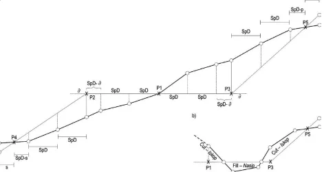
(5) Improving Accuracy in Earthwork Volume Estimation for Proposed Forest Roads ... (125–142). ì (BOP - PC ) 2 + (BOPY - PC Y (j + 1) ) 2 X X (j + 1) ï ï SDj = í ( PTX (j - 1) - PC X (j + 1) ) 2 + ( PTY (j - 1) - PC Y (j + 1) ) 2 ï 2 2 ïî ( PTX (j - 1) - EOPX ) + ( PTY (j - 1) - EOPY ). M. Contreras et al.. " j Î Q = {1} "j Î Q = {3, 5, 7, ... , ( 2n - 5)}. (13). "j Î Q = {2n - 3}. where, SDj is the horizontal distance of the jth road segment along the road centerline, and PTX(j–1), PTY(j–1), PTX(j+1), and PTY(j+1) are the x- and y-coordinates of the PT from the (j-1)th segment and the PC from the (j+1)th segment, respectively (Fig. 3). For straight segments, the model calculates the horizontal distance using the x- and y-coordinates of the previous curve PT and the following curve PC (Eq. 13). For the case of the first segment, the distance is calculated from BOP until the first curve PC, and the distance of the last segment is calculated from the last curve PT to EOP (Eq. 13, Fig. 3). For the case of curved segments, the model calculates the segment distance as follows: SDj = 2 × p × R ×. Dj 360. "j Î Q = {2, 4, 6, ... , ( 2n - 4)}. (14). where, SDj and Dj indicate the horizontal distance along the road centerline and the deflection of tangents in degrees associated with the jth curved segment, respectively (Fig. 3).. 2.4 Locating cross-sections for each road segment – Odre|ivanje popre~noga presjeka u svakom profilu ceste The model determines the number of cross-sections (CSN) for a given road segment based on the segment distance and a user-defined cross-section spacing (CSS). CSN for the jth road segment is then calculated by dividing SDj by CSS (Eq. 15). CSNj =. SDj CSS. , as a fractional notation. ì b > 0 Þ CSNj = a + 2 b CSNj = a if í c î b = 0 Þ CSNj = a + 1. (15). where, CSNj is the number of cross-sections on the jth road segment, a indicates the integer part of CSNj, b and c represent the numerator and denominator of the fractional part, respectively. When the horizontal distance of a road segment is shorter than CSS (SDj< CSS, thus a = 0), two cross-sections are located, one at the beginning and the other at the end of the road segment. All cross-sections along a road segment are located perpendicular to the road centerline. For the given jth road segment, the first cross-section is always located at the beginning of the road segment, the folCroat. j. for. eng. 33(2012)1. lowing cross-sections are spaced successively with an interval of CSS, and the last cross-section is always located at the end of the segment.. 2.5 Designing cross-sections – Kreiranje popre~nih presjeka For the purpose of comparing earthwork volumes estimated using different cross-section spacing, we simplified the cross-section design and made the following four assumptions: i) zero-line (balance point) is always located at half of the road width (RW), ii) road surface is flat, iii) road does not include a ditch, and iv) cut and fill slopes are constant. Fig. 4a presents the cross-section design considered in our model. For a given cross-section, horizontal distances from the road center (P1 in Fig. 4b) to its edges (P2 and P3 in Fig. 4b) are assumed to be fixed at RW/2. However, horizontal distances from P1 to the points where cut and fill slopes intersect with the ground profile (P4 and P5 in Fig. 4b) are variable because they depend on the ground slope. To obtain the design points necessary to draw a cross-section, the model first identifies the x-and y-coordinates of points P2 and P3 using the road width, the coordinates of P1, and the direction of the road segment mrs (Fig. 4b). The direction (mrs) is calculated differently for straight and curved segments (Eq. 16 and 17, respectively). ì PC Y (j + 1) - P1 Y "j Î Q = {1, 3, 5, ... , ( 2n - 5)} ï ï PC X (j + 1) - P1 X (16) mrs = í ï EOPY - P1 Y "j Î Q = {2n - 3} ïî EOP - P1 X X -1. æ CC Yj - P1 Y ö ÷ "j Î Q = 2, 4, 6, ... , ( 2n - 4) mrs = – ç { } ç CC Xj - P1 X ÷ ø è (17) where, CCXj and CCYj represent the x- and y-coordinates of CC associated with the jth curved road segment. The location of P2 and P3 are then calculated by adding or subtracting a difference in the x- and y-coordinates from the coordinates of the P1 (Eqs. 18–19).. 129.
(6) M. Contreras et al.. Improving Accuracy in Earthwork Volume Estimation for Proposed Forest Roads ... (125–142). Fig. 4 Cross-section design considered by the model (a), and road segment slopes (mrs) used to identify the location of cross-section design points on straight and curved road segments (b) Slika 4. Kreiranje popre~nog profila odre|enog modelom (a), te uzdu`ni nagib dionice {umske ceste (mrs) kori{ten za odre|ivanje osnovnih sastavnica popre~nog profila na ravnim dionicama te u horizontalnim kru`nim krivinama (b). PY = P1Y ±. ( RW / 2) 2 m +1 2 rs. PX = P1X + mrs × (P1Y–PY). (18) (19). where, the two pairs of and represent the locations of P2 and P3. To identify the locations of P4 and P5, the model iteratively places two points (Pt1 and Pt2 in Fig. 5) along the cross-section at a fixed distance interval, which is called span-distance (SpD) in our model. At iteration one, Pt1 starts at the edge of the road (P2 or P3 for the left or right side of the road, respectively), and Pt2 starts at meters away from Pt1 (Fig. 5). Thereafter, both points Pt1 and Pt2 are moved farther away from the road edge by SpD meters at each successive iteration. At a given iteration, the model calculates the x-, y-, and z-coordinates of Pt1 and Pt2 using the horizontal distances of Pt1 and Pt2 from P1. The model then checks whether the line formed between Pt1 and Pt2 intersects with the fill or cut slope line. The iteration process stops when the two lines intersect. Once this intersection point is known, the model calculates the horizontal distances (X_dist) from the road edge to P4 and P5 (Fig. 5). The model then calculates the two-dimensional coordinates of points P4 and P5 using Equations 18 and 19 replacing (RW/2) with (RW/2 + X_dist).. 130. 2.6 Calculating cut and fill areas – Izra~un povr{ine iskopa i nasipa To obtain ground elevations along a road cross-section, the model establishes ground points along the cross-section with an interval of SpD meters (Fig. 6a), and then estimates ground elevation on each point using the DEM and the interpolation method described in Section 2.1. The model then calculates cross-section areas (cut and fill) using a well-known. Fig. 5 Iterative process performed by the model to identify the intersection point (P5) between the cut slope and ground surface Slika 5. Postupak ponavljanja rada modela pri identificiranju to~ke sjeci{ta (P5) pokosa iskopa i terena Croat. j. for. eng. 33(2012)1.
(7) Improving Accuracy in Earthwork Volume Estimation for Proposed Forest Roads ... (125–142). æ CSS × TCA R ç ç TCA + TFA R R CVk = è 2 æ CSS × TCA R ç CSS ç TCA R + TFA R FVk = è 2. æ CSS × TCA L ö ÷ × TCA R ç ÷ ç TCA + TFA L L ø +è 2. ö ÷ × TCA L ÷ ø. æ ö CSS × TCA L ÷ × TFA R ç CSS ç ÷ TCA L + TFA L ø +è 2. ö ÷ × TFA L ÷ ø. M. Contreras et al.. (21). (22). where, CVk and FVk are the cut and fill volumes of the kth road section defined by two consecutive cross-sections. formula (Eq. 20), which provides the area of a polygon based on the coordinates of its vertices. This formula is derived from one half of the absolute value of the determinant of the matrix formed by the two-dimensional coordinates of the polygon vertices (Hush 1963). TPN. A = 0.5 × å [( xx p × z p + 1 ) - ( xx p + 1 × z p ) ]. (20). p =1. where, xxp is the horizontal distance from P1 to the pth point in the cross-section, zp is the elevation of the pth point, and TPN is the total number of points representing one side of the road from P1 where the area is calculated. Equation 20 provides cut or fill areas depending on whether all ground elevation. points are above or below the road surface. When both cut and fill areas are on one side of the road in the cross-section, where some ground elevation points are above the road surface and other points are below the road surface (Fig. 6b), the polygons representing either cut or fill are identified and their areas are calculated separately. Areas of the same type (cut or fill) are then added together to compute the total cut and fill areas for the right and left side of the road (TCAR, TFAR, TCAL, and TFAL respectively).. 2.7 Estimating cut and fill volumes – Procjena obujma zemljanih radova Based on our assumption that road centerlines are located at the ground level, earthwork volumes. Fig. 6 Cross-section design points used to calculate cut and fill areas (a), and an example of a cross-section having both fill and cut areas on one side of the road center line (P1) (b) Slika 6. Osnovne to~ke popre~noga profila kori{tene za izra~un povr{ina iskopa i nasipa (a) te primjer kada se s iste strane popre~noga profila nalaze povr{ine iskopa i nasipa (P1) (b) Croat. j. for. eng. 33(2012)1. 131.
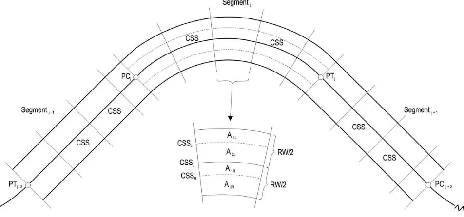
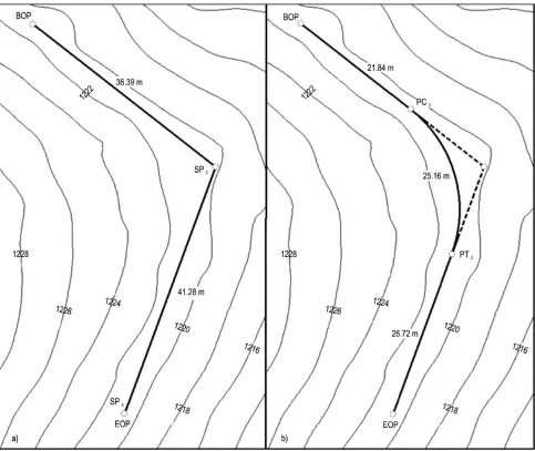
(8) M. Contreras et al.. Improving Accuracy in Earthwork Volume Estimation for Proposed Forest Roads ... (125–142). Fig. 7 Cross sections taken from straight and curved road segments for earthwork volume estimation Slika 7. Popre~ni presjeci na ravnim dionicama te u horizontalnim kru`nim lukovima ceste kao podloga za procjenu volumena zemljanih radova were estimated separately for each side of the road. For straight road segments we used the modified average end-area method developed by Epps and Corey (1990) to estimate earthwork volumes using the cut and fill areas of consecutive cross-sections (Eqs. 21–22) The CSS is the same on both sides of the road center line for straight road segments, whereas this is not the case for curved road segments (Fig. 7). For curved road segments, the model computes the actual cross-section spacing for each side of the road center line (CSSR and CSSL) separately by calculating the arc length of a curve whose radius makes the areas on both sides of the curve equal (A1R= A2R and A1L= A2L in Fig. 7). The arc lengths can be calculated as follows: R + (R ± RW /2) æ CSS × 360 × çç 2 R è 2. D=. 2. "j Î Q = {2, 4, 5, ... , ( 2n - 4)}. 2. ö ÷ ÷ ø. å CV. k. (24). k. (25). k =1. CSN - 1. FVj =. å FV k =1. Lastly, the total earthwork of the entire forest road is calculated by adding the total cut and fill volumes estimated for each road segment (Eqs. 26 and 27). 2 n-3. TCV =. å CV. j. (26). j. (27). j =1. 2 n-3. TFV =. å FV j =1. where, TCV and TFV represent the total cut and fill volumes of the entire road, respectively.. 3. Model applications – Primjena modela (23). where, the two values of D represent CSSR and CSSL. Once cross-section spacings along a curved road segment are obtained for both sides of the road center line, Equations 21 and 22 are used to estimate cut and fill volumes between consecutive cross-sections for curved road segments after CSS in the equation is replaced with CSSR and CSSL. Then, the total cut and fill volumes are calculated for the jth road segment using the following equations:. 132. CSN - 1. CVj =. 3.1 Verification – Provjera We created a hypothetical forest road to verify the results of our model and analyze the effects of using a high resolution DEM on earthwork volume estimates. We compared these estimates with those from the traditional method, which considers ground information only from pre-defined station points. The hypothetical road has three station points (Fig. 8a), resulting in two straight and one curved road segments (Fig. 8b). The hypothetical road was laid out Croat. j. for. eng. 33(2012)1.
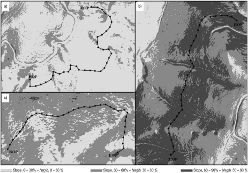
(9) Improving Accuracy in Earthwork Volume Estimation for Proposed Forest Roads ... (125–142). M. Contreras et al.. Fig. 8 Hypothetical forest road layout; a) station point locations, and b) road segment locations Slika 8. Polo`ajni nacrt hipotetske {umske ceste; a) polo`aj to~aka terenske izmjere, b) polo`aj dionica {umske ceste in the southern portion of the Mica Creek watershed located about 67 km southeast of Coeur d’Alene, Idaho, United States, where a LiDAR-derived, 1-meter resolution DEM is available. The road was manually digitized »on-screen« in ArcMap 9.2 based on a 2-meter contour lines layer derived from the DEM of the area. The ground slope in the area was moderate, ranging between 30 and 60%. We considered the following cross-section design and spacing parameters; cut slope (CS) = 1:1, fill slope (FS) = 1.5:1, road width (RW) = 4 m, radius of curve (R) = 20 m, and SpD = 1 m.. 3.2 Test case studies – Testiranje studije slu~aja To analyze the effects of various cross-section spacing on the accuracy of earthwork volume estiCroat. j. for. eng. 33(2012)1. mation, we created the layout of three hypothetical 1 km forest roads. These roads were located in areas with slopes between 0–30%, 30–60%, and 60–90% in the southern portion of the Mica Creek watershed to also examine the effects of ground steepness on earthwork volume estimation. We arbitrarily referred to these three areas with increasing slope as low, moderate, and steep terrain areas. The roads were manually digitized »on-screen« in ArcMap 9.2 based on 2-meter contour lines derived from the 1-meter resolution DEM of the area. The allowable road grade used the range from -15% to 15%. We assumed that 1-meter spacing provided the most accurate estimate, and used the earthwork volume obtained from 1-meter cross-section spacing as the true volume in comparison with other spacing. Fig. 9 illustrates the layout. 133.
(10) M. Contreras et al.. Improving Accuracy in Earthwork Volume Estimation for Proposed Forest Roads ... (125–142). Fig. 9 Layout of the three hypothetical 1 km forest roads located in low (a), moderate (b), and steep (c) slope areas Slika 9. Prikaz tri hipotetske {umske ceste projektirane na razli~itim kategorijama nagiba terena (a – 0 do 30 %, b – 30 do 60 % i c – 60 do 90 %) of the low, moderate and steep slope forest roads, which have 37, 36, and 37 station points, respectively. We also investigated the effect of terrain ruggedness on earthwork volume estimations. Most of the existing terrain ruggedness indexes calculated from ground elevation and aspect are designed to mea-. sure terrain heterogeneity for large areas using typically a 30 meter raster resolution (Riley et al. 1999, Sappington et al. 2007). When using a high-resolution 1-meter DEM, these indexes are not able to meaningfully capture terrain ruggedness for characterizing terrain variability along road segments. Therefore, we computed the coefficient of variation of the fill. Fig. 10 Number and location of cross-sections along a given straight road segment for different cross-section spacings (1, 2, 4, 8, and 16 meters) Slika 10. Broj i polo`aj popre~nih profila uzdu` ravne dionice {umske ceste za razli~ite ina~ice razmaka izme|u popre~nih profila (1, 2, 4, 8 i 16 metara) 134. Croat. j. for. eng. 33(2012)1.
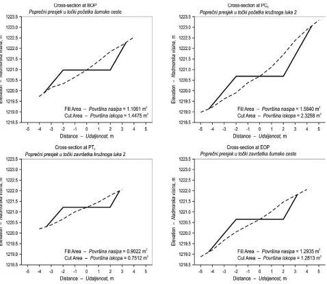
(11) Improving Accuracy in Earthwork Volume Estimation for Proposed Forest Roads ... (125–142). M. Contreras et al.. Fig. 11 Cross-section diagrams obtained for the 3-SP hypothetical forest road Slika 11. Crtani popre~ni profil u to~kama terenske izmjere na hipotetskim {umskim cestama and cut areas from all cross-sections in a given road segment, and used this coefficient of variation as a measure of terrain ruggedness in our study (e.g., the higher coefficient represents the more rugged terrain.) The coefficient was computed for all road segments included in the three hypothetical forest roads. Then, the road segments were grouped in three ranges of coefficient of variation: low (<20%), medium (20–40%), and high (³40%). The same parameter values used in the model verification regarding road design (RW and R), cross-section design (FS and CS), and spacing (SpD) were used for these applications. To make comparisons valid, specific cross-section spacings (e.g., 1, 2, 4, 8, 16 meters) were selected so that the same cross-sections can be used for smaller spacings analyzed (Fig. 10). Croat. j. for. eng. 33(2012)1. 4. Results and Discussion – Rezultati i rasprava 4.1 Model verification – Provjera modela Using the values of road design parameters specified above, we calculated cut and fill areas of each four cross-sections along the hypothetical forest road layout formed by two straight and one curve segment (see Fig. 8). Cut and fill areas for these cross-sections were also calculated manually to verify our model results (Fig. 11). Table 1 shows the coordinates of all cross-section design points as well as other points along the ground profile for each cross-section shown in Fig. 11. The results of area calculations from the model perfectly matched those calculated manually.. 135.
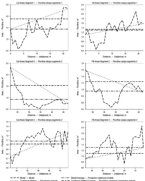
(12) M. Contreras et al.. Improving Accuracy in Earthwork Volume Estimation for Proposed Forest Roads ... (125–142). Table 1 X- and Z-coordinates calculated by the model to draw the cross-sections shown in Fig. 11 Tablica 1. Modelom izra~unate koordinate X i Z nacrtane na popre~nim profilima prikazanim na slici 11 BOP coordinates Koordinata po~etka ceste X1 Z2 –3.6234 1219.8796 –3.0000 1220.1448 –2.0000 1220.9619 –2.0000 1220.3194 –1.0000 1220.6205 0.0000 1220.9619 1.0000 1221.3924 2.0000 1220.9619 2.0000 1221.8531 3.0000 1222.1539 3.3107 1222.2726. PC2 coordinates Koordinata po~etka kru`noga luka 2 X1 Z2 –4.3041 1219.1348 –4.0000 1219.2062 –3.0000 1219.5960 –2.0000 1220.6709 –2.0000 1219.8930 –1.0000 1220.3587 0.0000 1220.6709 1.0000 1221.1097 2.0000 1220.6709 2.0000 1221.7045 3.0000 1222.3679 4.0000 1222.8951 4.3946 1223.0655. PT2 coordinates Koordinata zavr{etka kru`noga luka 2 X1 Z2 –3.3858 1220.2944 –3.0000 1220.3676 –2.0000 1221.2183 –2.0000 1220.6660 –1.0000 1220.9959 0.0000 1221.2183 1.0000 1221.4677 2.0000 1221.2183 2.0000 1221.7801 2.7864 1222.0046. EOP coordinates Koordinata zavr{etka ceste X1 Z2 –4.3221 1219.0900 –4.0000 1219.1963 –3.0000 1219.6519 –2.0000 1220.6380 –2.0000 1220.0318 –1.0000 1220.3419 0.0000 1220.6380 1.0000 1221.0162 2.0000 1220.6380 2.0000 1221.4700 3.0000 1221.7593 3.1738 1221.8119. 1. X-coordinate represents the horizontal distance in meters from P1 located at the origin of x-axis – koordinata X predstavlja horizontalnu udaljenost u metrima od sredi{nje osi ceste (apscisa slike 11) Z-coordinate represents elevation in meters – koordinata Z predstavlja nadmorsku visinu u metrima. 2. Table 2 Comparisons of cut and fill volumes estimated by the traditional method and the model Tablica 2. Usporedba procijenjenoga obujma zemljanih radova standardnom metodom i modelom Distance Udaljenost. Road gradient Nagib ceste. m. %. 1. 21.84. 2. 25.16. 3. 26.72. Totals – Ukupno. 73.72. –1.33 2.18 –2.17 –. Segment Nº Br. segmenta. 1. Traditional method – Stand. metoda Cut Volume Obujam iskopa. Fill Volume Obujam nasipa. Model – Model Cut Volume Obujam iskopa. Fill Volume Obujam nasipa. Difference – Razlika Cut Volume Obujam iskopa. m3 41.1984 38.7107 27.1596 107.0687. 29.3726 31.2789 29.3404 89.9919. Fill Volume Obujam nasipa. %1 31.0145 21.9750 28.8780 81.8676. 28.4278 25.0955 35.0607 88.5840. 32.84 76.16 –5.95 30.78. 3.32 24.64 –16.32 1.59. [(Traditional method – Model) / Model] * 100. Cut and fill volumes were estimated by our model using cross-sections placed every 1 meter. For the traditional method, we only considered the cross-sections located at the beginning and end of each road segment. Volume estimates varied widely between both methods (our model and the traditional method) for the three road segments, ranging from –6% to 76%, but the circular road segment presented the largest differences (Table 2). Cut and fill volumes were overestimated by the traditional method for road segments 1 and 2 (from 3 to 76%), and underestimated for the last road segment (from 6 to 16%). All in all, the traditional method overestimated the total cut and fill volumes for the 3-segment hypothetical forest road by 30% and 2%, respectively, when compared with the results of the model.. 136. Considerable variability in the cut and fill areas along the three road segments indicated that ground slopes along the road vary significantly (Fig. 12). This terrain variability caused the large differences in earthwork volume estimates between the two methods. While our model (by using 1-meter cross-section spacing) is able to capture details in terrain variations, these terrain details are ignored when only few cross-sections are considered in the traditional method. We also calculated the average value of the end areas resulted from the model and compared it with that from the traditional method (Fig. 12). The differences between the model average and the traditional method have a similar relationship as shown in the earthwork volume estimates presented in Table 2. This also suggests that the differences in earthCroat. j. for. eng. 33(2012)1.
(13) Improving Accuracy in Earthwork Volume Estimation for Proposed Forest Roads ... (125–142). M. Contreras et al.. Fig. 12 Cut and fill areas for the 3-SP hypothetical forest road calculated by the model and the traditional method Slika 12. Povr{ine iskopa i nasipa u to~kama terenske izmjere na hipotetskim {umskim cestama izra~unate modelom i standardnom metodom terenske izmjere Croat. j. for. eng. 33(2012)1. 137.
(14) M. Contreras et al.. Improving Accuracy in Earthwork Volume Estimation for Proposed Forest Roads ... (125–142). Fig. 13 Cut and fill volumes estimated by the model for the three hypothetical 1 km forest roads at different cross-section spacings Slika 13. Modelna procjena obujma iskopa i nasipa za tri hipotetske {umske ceste duljine po 1 km i za razli~ite razmake izme|u mjerenih popre~nih profila 138. Croat. j. for. eng. 33(2012)1.
(15) Improving Accuracy in Earthwork Volume Estimation for Proposed Forest Roads ... (125–142). work volumes between the two methods are caused by their different level of abilities to capture terrain variations. Due to the limitation in obtaining the »true« earthwork volume for a given road segment, it is impossible to properly verify our model for its earthwork volume estimation. However, our comparisons between the model results and the manual calculations of cut and fill area confirm that our model calculates correctly the earthwork volume and provides accurate estimates based on the assumption that the high resolution LiDAR-derived DEM provides an accurate representation of the ground surface.. 4.2 Test case studies – Testiranje studija slu~aja The model results of earthwork estimation for different cross-section spacings on the three hypothetical 1000-meter roads are presented and compared with the traditional method in Figure 13. A trend line was added to the estimated earthwork volumes from our model to show the pattern of changes in volume across different cross-section spacings. For the low slope hypothetical road, the traditional method (labeled as »Tra« in Fig. 13) overestimated both cut and fill volumes by 5.0% and 5.9%, respectively, compared with the results of the model with 1-meter cross-section spacing. For the moderate slope road, the traditional method underestimated cut volume by 1.7% but overestimated fill volume by 1.9%. In contrast, the traditional method overestimated cut volume by 2.2% but underestimated fill volume by 12.3% for the road located on steep terrain. The model results from different spacings show a general pattern indicating that as cross-section spacing increases, the earthwork volume estimates become closer to the volumes estimated by the traditional method. This is likely explained by the fact that, as cross-section spacing increases, the ability to capture terrain variations that may exist between consecutive cross-sections decreases, making the volume estimates become closer to those of the traditional method. Although the trend lines may suggest a relationship between the results of our model and the traditional method, no evidence of consistency in over- or underestimation of earthwork volumes was found. Cut and fill volumes were either overestimated or underestimated depending on the specific terrain conditions of road segments. Although Aruga et al. (2005) did not consider the same factors we did in this study, both studies realized that distance between cross-stations is important for accurately estimating earthwork volume. The shorter the distance, the larger ability we have in describing ground variability along the road lay out. Thus, it may be possible to estimate earthwork voluCroat. j. for. eng. 33(2012)1. M. Contreras et al.. me more accurately with short distances between cross-sections. The results of earthwork estimation for the three ranges of terrain ruggedness are presented in Fig. 14. The number of road segments included in each terrain ruggedness class (coefficient of variation) is different. Therefore, to compare the three terrain ruggedness classes, we plotted the average cut and fill volume per linear meter of road for each cross-section spacing used by the model and the traditional method. As expected, the model results of cut and fill volume estimation were similar to the results of the traditional method on the road segments that have a low coefficient of variation. For road segments that are in the medium class of coefficient of variation, the difference in cut volume estimates between the model and the traditional method was minor, but fill volumes estimated by the traditional method were 13% lower than the model results with 1-meter cross section spacing. Lastly, for the road segments with high coefficient of variation (highly rugged terrain), the traditional method overestimated cut volumes by 10.4%, while it underestimated fill volumes by 20.9%. In general, it is noticed that the differences in earthwork volume estimates between our model and the traditional method become larger as terrain ruggedness increases. Previous studies conducted by Aruga et al. (2005) and Akay (2003) also highlighted the importance of short distances between cross-sections in improving the accuracy of earthwork volume calculation, which is consistent with our findings in this study. The more rugged is the terrain where a forest road is laid out, the more important it would be to set out cross-sections in short distances in order to obtain an accurate estimation of earthwork volume. We recognize, however, that surveying a large number of cross-sections in the field might be a time-consuming task. We hope that the use of our model coupled with a high-resolution DEM can help improve the accuracy in earthwork volume estimation without much additional field work.. 5. Conclusions – Zaklju~ci In this study, we developed a computerized model to accurately estimate earthwork volumes of low-volume forest roads using a high-resolution DEM, and analyzed the effects of cross-section spacing on the accuracy of earthwork volume estimates. Although the accuracy of earthwork is expected to increase as cross-section spacing is reduced, to our knowledge, our model is the first attempt to quantify the differences between methods using ground information only at station points (the average meth-. 139.
(16) M. Contreras et al.. Improving Accuracy in Earthwork Volume Estimation for Proposed Forest Roads ... (125–142). Fig. 14 Cut and fill volumes estimated by the model for the road segments classified into three terrain ruggedness classes across different cross-section spacings Slika 14. Modelna procjena obujma iskopa i nasipa dionica {umske ceste razdijeljenih u tri kategorije neujedna~enosti terena za razli~ite razmake izme|u mjerenih (procijenjenih) popre~nih profila 140. Croat. j. for. eng. 33(2012)1.
(17) Improving Accuracy in Earthwork Volume Estimation for Proposed Forest Roads ... (125–142). od) and using high resolution DEM. When ignored, large terrain variations along road segments, as evidenced by the calculations of cut and fill areas from cross-sections spaced every 1meter, resulted in significant earthwork estimation errors. Our model offers a tool to help forest engineers to rapidly assess alternative forest road layouts and assist with planning activities to ensure the economic efficiency of forest road construction. The model verification and application results correspond with previous studies (Kim and Schonfeld 2001, Aruga et al. 2005) in terms of the relationship between accuracy and cross-section spacing. Assuming that 1-meter cross-section spacing provides the »true« earthwork volumes, the accuracy of earthwork volume estimates decreases with the increase of cross-section spacing. Moreover, the discrepancies in earthwork volume estimates between our model and the traditional end-area method become larger in more rugged terrain. Consequently, short cross-section spacing should be used to capture terrain variations and estimate earthwork volume more accurately when forest roads are planned and located on mountainous and rugged terrain. Several assumptions regarding cross-section design were made to simplify the estimation of areas and volumes as described in the method section. Although such assumptions may not seem practical, they do not affect our purpose of comparing earthwork volumes estimated at different cross-section spacings. In addition, the model can be further improved to consider real-world forest road survey and design practices.. 6. References – Literatura Akay, A., 2003: Minimizing total cost of construction, maintenance, and transportation costs with computer-aided forest road design. PhD dissertation in Forest Engineering. Oregon State University. 229p. Aruga, K., Sessions, J., Akay, A. E., 2005: Application of an airborne laser scanner to forest road design with accurate earthwork volumes. Journal of Forest Research 10: 113–123.. M. Contreras et al.. Coulter, E. D., Chung, W., Akay, A. E., Sessions, J., 2001: Forest road earthwork calculations for linear road segments using a high resolution digital terrain model generated from LiDAR data. In: Proceedings of the first precision forestry symposium. University of Washington, College of Forest Resources. Seattle, Washington, USA. June 17–20, 2001, 125–129. Easa, S. M., 1992a: Modified prismoidal method for nonlinear ground profiles. Surveying and Land Information Systems 52(1): 13–19. Easa, S. M., 1992b: Estimating earthwork volumes of curved roadways: Mathematical model. Journal of Transportation Engineering 118: 834–849. Epps, J. W., Corey, M. W., 1990: Cut and fill calculations by modified average-end-area-method. Journal of Transportation Engineering 116(5): 683–689. Hickerson, T. F., 1964: Route location and design. New York, McGraw-Hill, 5th edition Hush, B., 1963: Forest mensuration and statistics. Ronald Press Co, New York. 474p. Kim, E., Schonfeld, P., 2001: Estimating highway earthwork cross sections by using vector and parametric representation. Transportation Research Record 1772: 48–54. Paper No 01-2682 Reutebuch, S. E., McGaughey, R. J., Andersen, H., Carson, W. W., 2003: Accuracy of a high-resolution digital terrain modelunder a conifer forest canopy. Canadian Journal of Remote Sensing 29(5): 527–535. Riley, S. J., DeGloria, S. D., Elliot, R., 1999: A terrain ruggedness index that quantifies topographic heterogeneity. International Journal of Science 5: 1–4. Sappington, J. M., Longshore, K. M., Thompson, D. B., 2007: Quantifying landscape ruggedness for animal habitat analysis: A case study using bighorn sheep in the Mojave desert. The Journal of Wildlife Management 71(5): 1419–1426. Stückelberger, J., Heinimann, H., Burlet, E., 2006: Modeling spatial variability in the life-cycle costs of low-volume forest roads. European Journal of Forest Research 125(4): 377–390.. Sa`etak. Pobolj{anje to~nosti procjene zemljanih radova za predlo`ene {umske ceste primjenom digitalnoga modela terena visoke rezolucije Zemljani su radovi (radovi na donjem ustroju) najve}i tro{ak pri izgradnji {umskih cesta maloga prometnoga optere}enja i ~ine oko 80 posto ukupnih tro{kova izgradnje. To~nost procjene obujma zemljanih radova prijeko je potrebna pri procjeni tro{kova izgradnje {umskih cesta, racionalizaciji i kontroli tro{kovne sastavnice te pri. Croat. j. for. eng. 33(2012)1. 141.
(18) M. Contreras et al.. Improving Accuracy in Earthwork Volume Estimation for Proposed Forest Roads ... (125–142). izgradnji i uspostavi ekonomski u~inkovite primarne {umske prometne infrastrukture. Koli~ina se zemljanih radova kod {umskih cesta uobi~ajeno temelji na procjeni podataka dobivenih terenskom izmjerom na trasi {umske ceste. Povr{ina popre~nih profila procjenjuje se u svakoj to~ki izmjere, a zatim se klasi~ne metode, kao {to su metoda prosje~nih povr{ina ili metoda prizme, primjenjuju za izra~un obujma zemljanih radova izme|u susjednih popre~nih profila. Navedene metode pretpostavljaju jednoli~an teren izme|u popre~nih profila, {to pri kona~noj procjeni rezultira nedovoljno to~nim podacima u brdskim i planinskim podru~jima. U ovom je istra`ivanju razvijen ra~unalni model pobolj{ane to~nosti procjene zemljanih radova na {umskim cestama primjenom visoko razlu~iva digitalnoga modela terena. Istra`ivan je utjecaj udaljenosti izme|u profila na to~nost procjene obujma zemljanih radova primjenom predlo`enoga ra~unalnoga modela. Istra`ivane se {umske ceste nalaze u razli~itim reljefnim podru~jima, a prikazane su specifi~nim terenskim ~imbenicima te procjenom koli~ine zemljanih radova za razli~ite razmake izme|u profila. Analiziran je utjecaj razmaka izme|u popre~nih profila na to~nost procjene koli~ine zemljanih radova. Nadalje, utvr|ena je varijabilnost povr{ina popre~nih profila koja je kori{tena kao mjera nejednolikosti terena te su istra`eni i u~inci spomenute varijabilnosti na to~nost procjene obujma zemljanih radova. Izra|eni je ra~unalni model primijenjen na trima hipotetskim {umskim cestama na terenima nagiba <30 %, 30–60 % i 60–90 %, a procjena obujma zemljanih radova dobivenih modelom uspore|ena je sa standardnom metodom povr{ina u to~kama terenske izmjere. Op}enito gledaju}i, rezultati pokazuju kako pove}anje razmaka izme|u popre~nih profila smanjuje to~nost procjene obujma zemljanih radova zbog nemogu}nosti uzimanja u obzir nejednolikosti terena. Utvr|ene su razlike u procjeni obujma zemljanih radova izme|u predlo`enoga modela i klasi~nih metoda u rasponu od 2 do 12 % neovisno o nagibu terena. Jasniji je smjer primije}en kada se uspore|uju procjene obujma zemljanih radova predstavljenim ra~unalnim modelom u odnosu na standardne metode. Pove}anje nejednolikosti terena proporcionalno utje~e na razliku uspore|enih metoda u rasponu od 2 % na jednolikim terenima (izra`eno niskim koeficijentom varijacije povr{ine profila) pa do 21 % na nejednolikim terenima (izra`eno visokim koeficijentom varijacije povr{ine profila). Klju~ne rije~i: {umske ceste, obujam zemljanih radova, projektiranje cesta, LiDAR, digitalni model terena. Authors’ address – Adresa autorâ: Asst. Prof. Marco A. Contreras, PhD. e-mail: [email protected] University of Kentucky College of Agriculture Department of Forestry KY40546-0073 Lexington Thomas Poe Cooper Building 214 USA. Received (Primljeno): September 15, 2011 Accepted (Prihva}eno): February 21, 2012. 142. Pablo Aracena, Graduate Research Assistant e-mail: [email protected] Assoc. Prof. Woodam Chung, PhD. e-mail: [email protected] University of Montana College of Forestry and Conservation Department of Forest Management MT59812 Missoula USA Croat. j. for. eng. 33(2012)1.
(19)
Figure

+7

Related documents
