J.-S. Dhersin, Editor
NUMERICAL METHODS FOR PIECEWISE DETERMINISTIC MARKOV
PROCESSES WITH BOUNDARY
Ludovic Gouden`
ege
1Abstract. In this paper is described the general aspect of a numerical method for piecewise de-terministic Markov processes with boundary. Under very natural hypotheses, a crucial result about uniqueness of solution of a generalized Kolmogorov equation with respect to a test function space is proved. Next we prove the existence and uniqueness of a positive solution to the finite volume scheme without result about convergence. Finally different models of transmission control protocol window-size processes are simulated to illustrate the efficiency of the numerical method for describing the evolution of the density of a piecewise deterministic Markov process with boundary. Obviously some technical aspects have been skipped for reader convenience but the full theory will be exposed in a forthcoming paper in collaboration with C. Cocozza-Thivent1
, R. Eymard1
and M. Roussignol1
.
1.
Introduction
Piecewise Deterministic Markov Processes (PDMP) appear in many areas, such as engineering, operations research, biology, economics... One can find the definition and many properties of these processes in the founding book of M.H.A. Davis [8]. Relations between PDMP without boundary and point processes are developed in the book of M. Jacobsen [13]. Recently C. Cocozza-Thivent has deeply investigated relations between PDMP and Markov renewal theory [3] and extended PDMP’s definition. In all application areas most of interest quantities depend on the distribution of the process at each time, so it is essential of knowing how to compute these marginal distributions. The method proposed here consists in solving numerically equations which are fulfilled by the marginal distributions, namely generalized Kolmogorov equations. The characterization of the marginal distributions by these equations is studied in [5] for a PDMP without boundary. Finite volume schemes are proposed in [2, 4, 6, 10–12, 14].
One studies the following class of PDMP with boundary. The state space of the process is an open subsetF
of Rd and there exists a subset Γ of the topological boundary ofF which will force the process to jump. The
process (Xt)t≥0is a jump stochastic process onF whose trajectories are deterministic between the jump times. The deterministic trajectories are determined by a flow φ(x, t): if between s and t (s < t) the process does not reach the frontier and does not jump, then Xt =φ(Xs, t−s). Of course the flow has the “Markov property”φ(φ(x, s), t) =φ(x, s+t) as far as the boundary is not reached. Two kinds of jumps can occur. First there are stochastic jumps from a position x ∈ F with a jump rate λ(x) and a jump distribution Q(x,dy). Second when the process reaches a pointxof the boundary Γ, it jumps insideF with the distributionq(x,dy). Roughly speaking, these two kinds of jumps have different characters. The first ones occur at random times with probability density functions while the second ones occur at times with Dirac distributions.
1 Laboratoire d’Analyse et de Math´ematiques Appliqu´ees (CNRS - UMR 8050) Universit´e Paris-Est, 5 boulevard Descartes Champs sur Marne, 77454 Marne-la-Vall´ee Cedex 2, France
c
EDP Sciences, SMAI 2014
We assume the following notations and hypotheses on the data, denoted by (H) in this paper.
(1) d∈N⋆ andP(Rd) is the set of probability measures onRdwith borelian algebra,P(A) is the subset of
P(Rd) with support inAfor any measurable subsetA⊂Rd.
(2) The flowφ : Rd×R+→Rd is assumed to be such that:
(a) φ : Rd×R+→Rd is Lipschitz continuous with constantLφ,
(b) φ(x,0) =xfor allx∈Rdand
∀x∈Rd,∀t, s∈R+, φ(φ(x, t), s) =φ(x, t+s)
(c) LetF ⊂Rd be a non empty open set and G=Rd\F the complementary ofF be a non-empty closed set such that, for allx∈ Rd, there existst ∈ R+ such that φ(x, t) ∈G . We then define
α : Rd →R+by
α(x) = inf{t≥0, φ(x, t)∈G}.
Note that, for allx∈G,α(x) = 0, and that, for allx∈F, since φis continuous andGis closed,
α(x)>0. Note that the following property holds
∀x∈F, ∀t∈(0, α(x)), α(φ(x, t)) =α(x)−t.
We assume that the functionαis Lipschitz continuous with constantLα.
(d) We then denote Γ ={φ(x, α(x)), x∈F}. We have Γ⊂G. We cannot state whether Γ is open or closed.
(3) The transition rate λis such that λ∈Cb(F,R+), where Cb(F,R+) denotes the set of continuous and
bounded functions fromF toR+. We denote by Λ>0 a bound ofλ.
(4) The transition probabilityQ : F → P(F) (we then denote it byx7→Q(x,dy)) is such that: (a) there exists a functionfQ : R+→R+ such that
fQ(r) = sup x∈F
Z
{y∈F:|y|≥|x|+r}
Q(x,dy) and lim
r→∞fQ(r) = 0.
(b) for allξ∈Cb(F,R), the functionx→Rξ(y)Q(x,dy) is continuous fromF toR.
(5) The transition probabilityq : Γ→ P(F) (we then denote it byx7→q(x,dy)) is such that: (a) there exists a functionfq : R+→R+ such that
fq(r) = sup x∈Γ
Z
{y∈F:|y|≥|x|+r}
q(x,dy) and lim
r→∞fq(r) = 0.
(b) for allξ∈Cb(F,R), the functionx→Rξ(y)q(x,dy) is continuous from Γ toR.
(c) denoting 0 = exp(−B∞) for allB >0, we assume that there exists a0 ∈(0,1) andB0 >0 such that
sup x∈Γ
Z
F
e−B0α(y)q(x,dy)≤1−a
0.
(6) We assume thatρini∈ P(F) is given.
These hypotheses are very natural because we only assume Lipschitz continuous regularity. However some controls (especially hypothesis (H.5c)) are technical and could certainly be modified to be more general. In general, the flow φ is more regular as solution of an ordinary differential equation of the form ∂tφ(x, t) =
space) with desired properties. The regularity in hypotheses (H.4b) and (H.5b) are very natural, and again the state space could certainly be modified in order to satisfy these hypotheses. In general Q is absolutely continuous with respect to the Lebesgue measure such that for allx∈F there existshx a function onF such that Rξ(y)Q(x,dy) =R ξ(y)hx(y) dy for allξ∈Cb(F,R), then the regularity is transferred to the density hx.
The hypothesis is now verified for a bounded continuous functionx7→hx.
The distributionsρt∈ P(F) of the process at timetsatisfy the generalized Kolmogorov equation
Z
F
g(x, T)ρT( dx) =
Z
F
g(x,0)ρini( dx) +
Z
F×[0,T)
∂t,φg(x, t)µ( dx,dt) (1)
+
Z
F×[0,T)
λ(x)
Z
F
g(y, t)Q(x,dy)−g(x, t)
µ( dx,dt)
+
Z
Γ×[0,T)
Z
F
g(y, t)q(x,dy)−g(x, t)
σ( dx,dt), ∀g∈ T
where µ( dx,dt) =ρt( dx) dt. The measure σ, the test function spaceT and the operator∂t,φ are defined in Section 2. The measureσ describes the average number of times that the trajectories reach some parts of the boundary.
2.
Uniqueness
In the following, we propose a numerical scheme in order to compute numerically solutions of equation (1). A result of uniqueness is essential and needs an adapted test function space. This leads to the following definition.
Let us denote by Cc
b(Rd×R+) the set of allg ∈Cb(Rd×R+) with compact support in time, meaning that there exists T ∈R+(depending on g) such thatg(x, t) = 0 for allt≥T.
For allg∈Cc
b(Rd×R+), let:
∂t,φg(x, t) = lim sup n→∞
g(φ(x,1/n), t+ 1/n)−g(x, t) 1/n
when this limit is finite and 0 if not. The operator ∂t,φ is called the derivation along the flow. If ∂tg(x, t) = limǫ→0g(x,t+ǫ)−g(x,t)ǫ and∂φg(x, t) = limǫ→0g(φ(x,ǫ),t)−g(x,t)ǫ exist, then for all (x, t)∈Rd×R+and 0≤t < α(x) the functiont7→g(φ(x, t), t) is differentiable and∂t,φg(x, t) =∂tg(x, t) +∂φg(x, t).
Definition 2.1. We denote by T the set of all functions g ∈ Cc
b(Rd ×R+) such that there exists I, J ∈ Cc
b(Rd×R+) with
∀(x, t)∈Rd×R+, g(x, t) =J(φ(x, α(x)), t+α(x))−
Z α(x)
0
I(φ(x, s), t+s) ds.
We then denoteg=T(I, J).
We will useT as test function space in the proof of uniqueness. Ifg=T(I, J)∈ T, it is easy to verify that forx∈Gwe haveg(x, t) =J(x, t) and that forx∈F and 0< ǫ < α(x) we have
g(φ(x, ǫ), t+ǫ)−g(x, t) =
Z ǫ
0
I(φ(x, s), t+s) ds.
Then, for all g =T(I, J)∈ T and for allx∈F andt ∈R+, we have I =∂t,φg. Hence, for given I, J,I,eJe∈
Cc
Definition 2.2. We say that non negative measuresµand σsuch that∀ T ∈R+, µ(F×[0, T])<∞, σ(Γ×
[0, T])<∞, µ((Rd\F)×R+) = 0 andσ((Rd\Γ)×R+) = 0 are solutions of ProblemPif for allg=T(I, J)∈ T
0 =
Z
F
g(x,0)ρini( dx) +
Z
F×R+
I(x, t)µ( dx,dt)
+
Z
F×R+
λ(x)
Z
F
g(y, t)Q(x,dy)−g(x, t)
µ( dx,dt) (2)
+
Z
Γ×R+
Z
F
g(y, t)q(x,dy)−g(x, t)
σ( dx,dt).
We have the following uniqueness result.
Theorem 2.3. Under hypotheses (H), there exists at most a unique couple (µ, σ)solution of Problem P. Proof. Suppose there exist two solutions (˜µ,σ˜) and (ˆµ,σˆ) to ProblemP. Denote (¯µ,σ¯) the measures such that ¯
µ= ˜µ−µˆand ¯σ= ˜σ−σˆ. Then for allg=T(I, J)∈ T, we have
0 =
Z
F×R+
I(x, t)¯µ( dx,dt)
+
Z
F×R+
λ(x)
Z
F
g(y, t)Q(x,dy)−g(x, t)
¯
µ( dx,dt)
+
Z
Γ×R+
Z
F
g(x, t)q(z,dx)−g(z, t)
¯
σ( dz,dt).
LetI, J∈Cc
b(Rd×R+). Using Lemma 2.4, we can findI, J∈Ccb(Rd×R+) such thatg=T(I, J) verifies
∀(x, t)∈Rd×R+, I(x, t) =I(x, t) +λ(x) Z
F
g(y, t)Q(x,dy)−g(x, t)
,
and ∀(z, t)∈Rd×R+, J(z, t) = Z
F
g(x, t)q(z,dx)−J(z, t).
Thus the measures ¯µand ¯σverify
Z
F×R+
I(x, t)¯µ( dx,dt) +
Z
Γ×R+
J(z, t)¯σ( dz,dt) = 0.
Since this equality is verified for all ¯I,J¯∈Cc
b(Rd×R+), it proves that the measures ¯µand ¯σvanish. The previous proof uses the following lemma which is an original result. In fact, this is the core of the problem and it has given to the author a good representation for the spaceT of test functions. Moreover many hypotheses are used in this lemma and the reader can understand the choice of hypothesis by reading this proof, in particular it explains the form of hypothesis (H.5c).
Lemma 2.4 (Operator’s inversion). Under hypotheses (H), let I, J ∈Cc
b(Rd×R+). Then there exists I, J ∈ Ccb(Rd×R+)such that, settingg=T(I, J), we have
∀(x, t)∈Rd×R+, I(x, t) =I(x, t) +λ(x) Z
F
g(y, t)Q(x,dy)−g(x, t)
, (3)
and
∀(z, t)∈Rd×R+, J(z, t) = Z
F
Proof. There existsT >0 such thatI(x, t) =J(x, t) = 0 for allx∈Rd andt≥T. Let
CT
b ={g∈Cb(Rd×R+), ∀(x, t)∈Rd×[T,+∞[, g(x, t) = 0}.
Remark that it is clear that for all I, J ∈ CT
b, T(I, J)∈CTb. We define αT(x) = min(α(x), T) for allx∈Rd and a norm on CT
b by
∀g∈CTb, kgkA,B:= sup (x,t)∈Rd×[0,T]
exp(BαT(x) +At) |g(x, t)|,
for givenA, B >0 chosen later. CT
b is a Banach space with this norm. Then we define a sequence of functions (In, Jn)n∈
Nsuch thatI0=J0= 0 and for alln∈N
∀(x, t)∈Rd×R+, In+1(x, t) =I(x, t)−λ(x) Z
F
T(In, Jn)(y, t)Q(x,dy)−T(In, Jn)(x, t)
,
∀(z, t)∈Rd×R+, Jn+1(z, t) = Z
F
T(In, Jn)(x, t)q(z,dx)−J(z, t).
This define a sequence (T(In, Jn))n∈N in CTb whereT(In+1, Jn+1) = Ψ(T(In, Jn)) for an obvious operator Ψ .
Let us prove that this sequence converges. For this, it is sufficient to prove that the operator Ψ is really well defined and there existsk∈(0,1) such that for all (I, J)∈(CT
b)2 and (I′, J′)∈(CTb)2 we have
kΨ(T(I, J))−Ψ(T(I′, J′))kA,B≤kkT(I, J)−T(I′, J′)kA,B.
Then, using the definition of (In+1, Jn+1), we get that the sequence (In, Jn)n∈
N is convergent as well. The
limit satisfy (3) and (4).
Let us setf =T(I−I′, J−J′), let (x, t)∈Rd×[0, T]. We have
(Ψ(T(I, J))−Ψ(T(I′, J′))) (x, t) =T1−T2+T3,
with
T1=
Z αT (x)
0
λ(φ(x, s))
Z
F
f(y, t+s)Q(φ(x, s),dy) ds,
T2=
Z αT (x)
0
λ(φ(x, s))f(φ(x, s), t+s) ds, and T3=
Z
F
f(y, t+α(x))q(φ(x, α(x)),dy).
We then have
|T1| ≤
Z αT (x)
0
exp(−A(t+s))λ(φ(x, s))
×
Z
F
exp(A(t+s)) exp(−BαT(y)) exp(BαT(y))f(y, t+s)Q(φ(x, s),dy) ds
≤
Z αT (x)
0
exp(−A(t+s))|λ(φ(x, s))|
Z
F
exp(−BαT(y))kfkA,BQ(φ(x, s),dy) ds
≤ kfkA,B
Z αT (x)
0
exp(−A(t+s))|λ(φ(x, s))|ds.
Therefore we get
exp(At+BαT(x))|T1| ≤ kfkA,B
Z αT (x)
0
exp(−As)|λ(φ(x, s))|exp(BαT(x)) ds≤ kfkA,BΛ exp(BT)
In the same way, assumingA > B and using α(φ(x, s)) =α(x)−swhich leads to αT(φ(x, s))≥αT(x)−s,
exp(At+BαT(x))|T
2| ≤ ΛkfkA,B 1
A−B.
Finally, forA > B, usingf(y, t+α(x)) =f(y, t+αT(x)) for all (y, t)∈Rd×R
+ for allx∈Rd, we have
exp(At+BαT(x))|T3| ≤ kfkA,B
Z
F
exp(−Bα(y))q(φ(x, α(x)),dy) + exp(−BT)
.
Finally we need to choose sufficiently large constantsAandB withA > B such that
sup x∈Rd
Λ exp(BT)
A +
Λ
A−B +
Z
F
exp(−Bα(y))q(φ(x, α(x)),dy) + exp(−BT)
≤k <1.
Thanks to Hypothesis (H.5c), setting first largeB and next largeA, we obtain the result fork= 1−a0
2 <1. So it only remains to prove that the operator Ψ is well defined such that it effectively mapsT ∩CT
b toT ∩CTb. Remark that it is sufficient to prove that the following terms (Ui)i=1..5 are in CT
b.
U1:=
Z α(x)
0
I(φ(x, s), t+s) ds, U2:=
Z α(x)
0
λ(φ(x, s))
Z
F
T(I, J)(y, t+s)Q(φ(x, s),dy) ds,
U3:=
Z α(x)
0
λ(φ(x, s))T(I, J)(φ(x, s), t+s) ds,
U4:=
Z
F
T(I, J)(y, α(x) +t)q(φ(x, α(x)),dy) and U5:=J(φ(x, α(x)), α(x) +t).
First remark that all terms are bounded since
|U1| ≤TkIk∞, |U2|+|U3| ≤2TΛkT(I, J)k∞, |U4| ≤ kT(I, J)k∞ and |U5| ≤ kJk∞.
Moreover, for all t > T, all terms vanish. So it only remains to prove the continuity. Since I, J, φ and α
are continuous, U1 and U5 are clearly continuous. U3 is clearly continuous since λ and T(I, J) are bounded continuous functions. Finally U2 andU4 are continuous too: it is relatively straightforward using Hypotheses
(H.4a), (H.4b), (H.5a) and (H.5b).
3.
A finite volume scheme
We now come to the presentation of the finite volume scheme, which has been used in [10] for the approxima-tion of a benchmark problem. Such schemes are not classically used in the framework of probabilistic studies, since they have mainly be developed by engineers, in order to approximate the solutions of balance equations. We then consider that (1) can be viewed as balance equations describing the conservation of probability. We then introduce the finite volume discretization by the following notations and definitions.
(1) We define a reference measure, denoted by dx or dy, on F, with respect to all borelian sets of Rd
restricted toF.
(2) An admissible mesh M of F is a countable partition of F, therefore such that ∪K∈MK = F and
∀(K, L)∈ M2, K=6 L⇒K∩L=∅.
(3) ∀K∈ M, |K|:=RK dx >0.
(4) sup K∈M
diam(K)<+∞where diam(K) = sup {(x,y)∈K2}
|x−y|. We then seth:= sup K∈M
diam(K).
The value τ > 0, aimed to tend to 0, is used for the definition, for all K ∈ M and L∈ M, of the flux of probability mass from Kto Lby
vKL=
1
τ|{x∈K:α(x)> τ andφ(x, τ)∈L}|. (5)
And∀(K, L)∈ M × Mwe define
λKL=
Z
K
λ(x)
Z
L
Q(x,dy)dx, λK=
Z
K
λ(x)dx= X
L∈M
λKL, (6)
qK =
1
τ|{x∈K:α(x)≤τ}|, and qKL=
1
τ
Z
{x∈K:α(x)≤τ}
Z
L
q(φ(x, α(x)),dy)dx. (7)
We may now define a familyp(K)n
n∈N,K∈M of real values thanks to the following finite volume scheme, which is time implicit.
|K|p
(K) n+1−p
(K) n
δt +
X
L∈M
vKLp(K)n+1−vLKp(L)n+1
+ (λK+qK)p(K)n+1−
X
L∈M
p(L)n+1(λLK+qLK) = 0, ∀K∈ M, ∀n∈N, (8)
with the initial condition
|K|p(K)0 =
Z
K
ρini(dx), ∀K∈ M. (9)
Let us remark that the following property holds:
τ X
L∈M
vKL+qK
!
=|K|, ∀K∈ M. (10)
Therefore, scheme (8) may be rewritten
1 +δt
τ
|K|+δtλK
p(K)n+1−δt
X
L∈M
p(L)n+1(vLK+λLK+qLK) =|K|p(K)n , ∀K∈ M, ∀n∈N. (11)
We then define the approximation µD( dx,dt) (resp. σD( dx,dt)) of the measureµ( dx,dt) on F×R+ (resp.
σ( dx,dt) on Γ×R+) by Z
Rd×R
+
f(x, t)µD( dx,dt) =X
n∈N
δt X
K∈M
p(K)n+1
Z
K
f(x, nδt)dx,
for all bounded continuous functionf ∈Cc b, and
Z
Rd ×R+
f(x, t)σD( dx,dt) =X
n∈N
δt X
K∈M
p(K)n+1 1
τ
Z
{x∈K:α(x)≤τ}
f(φ(x, α(x)), nδt)dx,
(1) An explicit version of the scheme could be defined, following the ideas of [6]. But the main drawback of an explicit scheme is that it cannot provide, in the general case, an approximation of the asymptotic marginal distributions at large times, with an acceptable computing cost.
(2) An implicit scheme has been provided in [11]. But in this scheme the considered flow is much more regular (it is assumed to be the solution of an EDO).
(3) An explicit scheme is introduced in [2] for Lipschitz flows. The present scheme uses the valueτ >0 in the same way as the time step is used in [2] (where the convergence of the scheme is proved for general Lipschitz flowφin the caseδt→0 andh/δt→0).
(4) In [10], the asymptotic states at large times have been obtained lettingδt→ ∞ in an implicit scheme. Hence it is interesting to use the parametershandτ which can tend to 0 independently ofδt.
Remark 3.1. Since (8) is an infinite linear system, the existence and uniqueness of a positive solution must be first addressed. From a numerical point of view, this infinite linear system should be treated with caution, but we often have a system with finite number of unknowns.
Lemma 3.2 (Existence of solution). Under Hypotheses (H) and numerical hypotheses, there exists one and only one solution(p(K)n )K∈M,n∈N to Scheme (5),(7),(6),(8),(9) which satisfies:
p(K)n ≥0, ∀K∈ M, ∀n∈N, (12)
P
K∈M|K|p (K)
n = 1, ∀n∈N. (13)
Proof. Let us first show the existence of a solution to the scheme. We consider the valuesp(K)(k) defined, for given
n∈Nand (p(K)n )K∈M such that (12)-(13), by:
p(K)(0) =p(K)n , ∀K∈ M,
1 + δt
τ
|K|+δtλK
p(K)(k+1)=δt X
L∈M
p(L)(k)(vLK+λLK+qLK) +|K|p(K)n , ∀K∈ M, ∀k∈N.
(14)
Denoting, fork∈NandK∈ M,pb(K)
(k+1)=p (K) (k+1)−p
(K)
(k), we have
1 + δt
τ
|K|+δtλK
b
p(K)(1) =δt X
L∈M
p(L)n (vLK+λLK+qLK)−
δt
τ|K|+δtλK
p(K)n , ∀K∈ M,
1 + δt
τ
|K|+δtλK
b
p(K)(k+1)=δt X
L∈M
b
p(L)(k)(vLK+λLK+qLK), ∀K∈ M,∀k∈N⋆.
We notice that, thanks to (10) and (13), we have
X
K∈M
1 + δt
τ
|K|+δtλK bp(K)(1)
≤2
δt
τ + Λδt
. and X K∈M
1 + δt
τ
|K|+δtλK bp(K)(k+1)
≤ X L∈M δt
τ|L|+δtλL
Then, by induction, we get that the valueuk =PL∈M δtτ|L|+δtλL
|pb(L)(k)|is positive and nonincreasing with respect to k∈N⋆. We then deduce that the sequence (uk)k∈N⋆ is convergent. Writing
X
K∈M
|K|bp(K)(k+1)≤uk−uk+1,
we deduce thatpb(K)(k+1)is the general term of an absolutely convergent series. Therefore the sequencep(K)(k+1)
k∈N
satisfying
p(K)(k+1)=p(K)n + k
X
m=0
b
p(K)(m+1),
converges to a value denoted byp(K)n+1. Passing to the limit in (14), we obtain that these values are solution to the scheme. Moreover, they satisfy that
X
K∈M
|K|p(K)(k) ≤1 +u1−uk ≤1 +u1.
Therefore we can sum (8) onK∈ M, obtaining by induction that (13) holds forn+ 1.
Remark 3.3. In the case of an infinite state space, we can consider a bounded subdomain ˜F to do the computation until the density reaches the boundary of ˜F. Next enlarge the subdomain ˜F and continue the computation. However, since the scheme is implicit, it could arrived after very few iteration.
Remark 3.4. The matrix representing the linear system is potentially completely full because many coefficients
λKL are strictly positive and there is no simple way to reduce the complexity of this system inversion. But we only need to compute a unique LU decomposition to do multiple iterations of the scheme, because it is time independent. Moreover the computation of the coefficients of the matrix vKL, λKL and qKL is not an easy problem, because there is numerical difficulties depending on the geometry of the mesh or the quadrature rule used for the approximation of integrals.
Let us now turn to the uniqueness of this solution. Denoting bypb(K)the difference between two solutions of (11), and using that the two solutions satisfy (12)-(13), one may write
1 + δt
τ
|K|+δtλK
|pb(K)| ≤δt X
L∈M
|pb(L)|(vLK +λLK+qLK), ∀K∈ M,
which provides, summing onK∈ M,
X
K∈M
1 +δt
τ
|K|+δtλK
|pb(K)| ≤ X
L∈M
δt
τ|L|+δtλL
|pb(L)|,
and thereforePK∈M|K||pb(K)|= 0. Hence the uniqueness proof.
Remark 3.5. Since we have proved that the scheme is well-posed, some numerical tests are described in the Section 4. But the convergence of the scheme needs some additional properties (whose proofs are not detailed here):
• finiteness of the mass σD(Γ×[0, T]),
• tightness of the family of probability measures (µD)D∈F given a familyF of discretizationsDverifying some restrictions likeh/τ ≤1,
4.
Numerical test and conclusion
Now we present different models in dimension d = 1 to illustrate the efficiency of the numerical method for describing the evolution of the density of a PDMP with (or without) boundary. We are interested in the Transmission Control Protocol (TCP) window size process (described in [9]). The first model is named the infinite maximum window size (TCP-I), the second model is a finite maximum window size (TCP-F) and the third model is a finite maximum window size with jump (TCP-FJ). In our framework, let the state space1
F be the interval (−∞, X) for given X > 0. Its complementary set G is [X,+∞). The flow is given by
φ(x, t) = min(x+t, X) for all (x, t)∈R×R+. It is clear thatα(x) =X−xfor allx∈F andα(x) = 0 for all
x∈G, so Γ ={X}. The jump rateλis an increasing function of the position, preciselyλ:x7→x+. Thus,“the higher a component is, the sooner it will jump”. Q(x,dy) is a Dirac measure on pointx/2 for allx∈F. These assumptions are common to the three models. For the TCP-I model, we takeX as large as possible such that it does not perturb the dynamics. For the TCP-F model, we take a finiteX and give no particular behavior at Γ. Finally for the TCP-FJ model, we take a finite X and force the process to jump. Precisely, at point {X}
the process jumps with probabilitypat point {X/2} and with probability 1−puniformly on (0, X) so
q(0,dy) =p δX/2(y) +1−p
X χ(0,X)(y) dy,
with obvious notations. Finally we chooseρinias the Dirac distribution at point{0}(the computer starts). The distributions ρT of this process at timeT satisfy the generalized Kolmogorov equation
Z
(−∞,X)
g(x, T)ρT( dx) =g(0,0) +
Z
(−∞,X)×[0,T)
(∂t+∂x)g(x, t)µ( dx,dt)
+
Z
(−∞,X)×[0,T)
x(g(x/2, t)−g(x, t))µ( dx,dt)
+
Z
[0,T)
p g(X/2, t) + (1−p)
Z
(0,X)
g(y, t) dy−g(X, t)
!
σ({X},dt), ∀g∈ T.
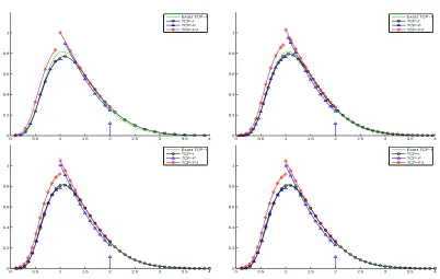
In [7] the authors get quantitative estimates for the convergence to equilibrium which suggest that an ex-ponential rate could be obtained in many variant of the TCP window size process. So we present the density at time T = 10 (the equilibrium is reached). For the simulation we have chosen X = 6 in the TCP-I model,
X = 2 in the TCP-F or TCP-FJ models andp= 0.5. We want to illustrate convergence ash, τ, δt→0. So we apply the numerical method with the mesh ∪K≤X/h[Kh−h, Kh[ for different parameters h, τ and δt= 0.01. Moreover we have drawn in solid line the explicit density of the TCP-I model given in [9]. Finally, for the TCP-F model, the asymptotic density has a Dirac mass at point X which is drawn as a vertical arrow whose height is its mass. The results are illustrated on Figure 1 on a common state space [0,4].
To conclude we say that the numerical method developed here for Piecewise Deterministic Markov Processes must now be tested on different PDMPs, some of them related to practical cases and others in order to un-derstand their behavior. Indeed the method permits to view the global behavior of the density, whereas the classical approach with particles and Monte-Carlo simulations only describes the trajectories. With our method we can see how the stochastic jumps interact with the flow, which leads sometimes to some unexpected behav-iors (see [1]). Moreover the method is robust with large values ofδt, which permits to compute the asymptotic stationary states of a PDMP.
Acknowledgement: The author is thankful for F. Nabet’s advice about finite volume simulations.
0 0.5 1 1.5 2 2.5 3 3.5 4 0
0.2 0.4 0.6 0.8 1
Exact TCP−I TCP−I TCP−F TCP−FJ
0 0.5 1 1.5 2 2.5 3 3.5 4 0
0.2 0.4 0.6 0.8 1
Exact TCP−I TCP−I TCP−F TCP−FJ
0 0.5 1 1.5 2 2.5 3 3.5 4 0
0.2 0.4 0.6 0.8 1
Exact TCP−I TCP−I TCP−F TCP−FJ
0 0.5 1 1.5 2 2.5 3 3.5 4 0
0.2 0.4 0.6 0.8 1
Exact TCP−I TCP−I TCP−F TCP−FJ
Figure 1. Densities for parameters (top-left)h=τ =δt= 0.2, (top-right) h=τ =δt= 0.1, (bottom-left)h=τ=δt= 0.01 and (bottom-right)h= 2τ =δt= 0.01.
References
[1] M. Bena¨ım, S. Le Borgne, F. Malrieu, P.-A. Zitt, (2013) Qualitative properties of certain piecewise deterministic Markov processes, arXiv:1204.4143v3.
[2] F. Bouchut, R. Eymard, A. Prignet (2011) Finite volume schemes for the approximation via characteristics of linear convection equations with irregular data,Journal of Evolution Equations, 11, 3 (2011) 687-724.
[3] C. Cocozza-Thivent (2013) Renouvellement markovien et PDMP, online at : http://perso-math.univ-mlv.fr/users/ cocozza.christiane/recherche-page-perso/PresentationRMetPDMP.html (in french).
[4] C. Cocozza-Thivent, R. Eymard (2004) Approximation of the marginal distributions of a semi-Markov process using a finite volume scheme,ESAIM: M2AN, vol. 38, n5, p. 853-875.
[5] C. Cocozza-Thivent, R. Eymard, S. Mercier, M. Roussignol (2006) Characterization of the marginal distributions of Markov processes used in dynamic reliability,Journal of Applied Mathematics and Stochastic Analysis, ID Article 92156, pp. 1-18. [6] C. Cocozza-Thivent, R. Eymard, S. Mercier (2006) A finite volume scheme for dynamic reliability models,IMA Journal of
Numerical Analysis,published online on Marsh 6, 2006, DOI:10.1093/imanum/drl001.
[7] D. Chafa¨ı, F. Malrieu, K. Paroux (2010) On the long time behavior of the TCP window size process,Stochastic Processes and their Applications, Volume 120, Issue 8 pp. 1518-1534.
[8] M.H.A. Davis (1993),Markov Models and Optimization, Chapman & Hall, London.
[9] V. Dumas, F. Guillemin, Ph. Robert, (2002) A Markovian analysis of additive-increase multiplicative-decrease (aimd) algo-rithms,Adv. in Appl. Probab.Volume 34, Issue 1, 85-111.
[10] R. Eymard, S. Mercier (2008), Comparison of numerical methods for the assessment of production availability of a hybrid system,Reliability Engineering & System Safety, Volume 93(1), 169-178.
[11] R. Eymard, S. Mercier, A. Prignet (2008) An implicit finite volume scheme for a scalar hyperbolic problem with measure data related to piecewise deterministic Markov processes,Journal of Computational and Applied Mathematics, 222(2), pp. 293-323. [12] R. Eymard, S. Mercier, M. Roussignol (2011), Importance and sensitivity analysis in dynamic reliability, Methodology and
Computing in Applied Probability, 13(1), pp. 75-104. DOI 10.1007/s11009-009-9122-x.
[13] M. Jacobsen (2006),Point process theory and applications: marked point and piecewise deterministic processes,Series: Prob-ability and Its Applications, Birkh¨auser.