AUT J. Elec. Eng., 50(2) (2018) 129-134 DOI: 10.22060/eej.2018.13944.5199
Improved Channel Estimation for DVB-T2 Systems by Utilizing Side Information on
OFDM Sparse Channel Estimation
S. Ghazi-Maghrebi1*, S. H. Hashemi-Rafsanjani2
1 College of Electrical Engineering, Islamic Azad University, Yadegar-e Imam Khomeini (RAH) Shahr-e Rey Branch, Tehran, Iran 2 Digital Communication, ICT Research Center, Tehran, Iran
ABSTRACT: The second generation of digital video broadcasting (DVB-T2) standard utilizes orthogonal frequency division multiplexing (OFDM) system to reduce and to compensate the channel effects by utilizing its estimation. Since wireless channels are inherently sparse, it is possible to utilize sparse representation (SR) methods to estimate the channel. In addition to sparsity feature of the channel, there is usually some additional information, known as side information. The side information, in general application, is not used in ordinary sparse channel estimation methods. However, utilizing the side information may help improve the channel estimation. In this paper, we utilize side information to estimate sparse channel of an OFDM system. Also, for more verification of the proposed method in this paper, we have shown the impact of side information in the estimation procedure for an applied system such as DVB-T2 system. Simulation results, in this research, show that utilizing side information not only increases the performance of the DVB-T2 system, but also releases a portion of resources of the system such as estimation-pilots. It is obvious that these resources can be used for increasing data rate.
Review History: Received: 18 January 2018 Revised: 13 June 2018 Accepted: 18 June 2018 Available Online: 1 July 2018
Keywords: DVB-T2 System Sparse Channel Estimation OFDM Modulation Side Information
1- Introduction
The second generation of digital video broadcasting (DVB-T2) [1] is the second version of digital video broadcasting standard which is published as EN 300 744 standard [1]. These systems utilize orthogonal frequency division multiplexing (OFDM) to modulate data. The OFDM modulation is a special type of multi-carrier modulation which utilizes Fast Fourier Transform (FFT) and Inverse Fast Fourier Transform (IFFT) blocks to multiplex digital data at orthogonal sub-carriers [2, 3]. This method is used to overcome multipath effects of wireless channels. For this purpose, the receiver side should have an estimation of the channel to compensate channel effects [4]. Therefore, channel estimation is a crucial part of the OFDM modulation-based system. Different approaches in the literature [5-9] are suggested to provide reliable estimation while reducing the computational complexity of the system.
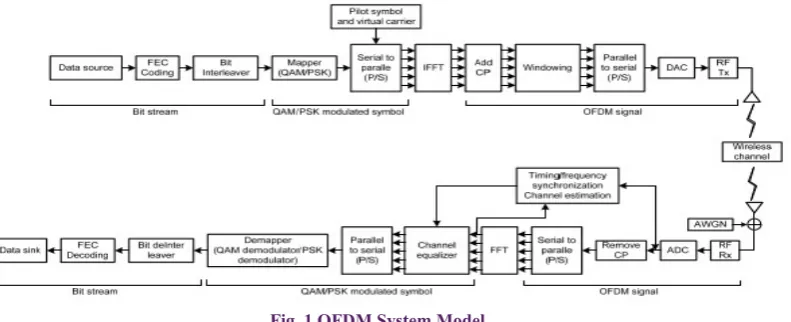
The OFDM channel estimation approach can be categorized into two different classes or methods, namely Training Based Sequence (TBS) and Pilot Based Sequence (PBS) [2]. The TBS method utilizes an OFDM symbol to estimate the channel for a block of OFDM symbols. On the other hand, the PBS method, as indicated in figure (1), is commonly used for estimating the channel for each OFDM symbol by employing some pilots known as estimation pilots [2, 10]. This method prepares an OFDM symbol by appending estimation pilots to data samples. A stream of OFDM symbols is passed through an IFFT block. Then, for compensating inter symbol interference (ISI), a copy of a part of the OFDM symbol known as cyclic prefix (CP), is appended to each symbol and prepares OFDM symbol to transmit. These symbols are transmitted consecutively through a wireless channel [2].
At the receiver side, the appended guard-band is removed and the rest of the symbol is forwarded to the FFT block. The receiver estimates the channel by utilizing samples of the channel frequency response which are obtained from the estimation pilots [2]. Note that the received samples are always contaminated by noise. In order to combat the effect of noise, some estimation methods try to utilize the time and frequency coherence of the channel which is optimally obtained by applying two dimensional filters [11]. For example, the authors in [12] proposed applying two one-dimensional filters to extract time and frequency coherence instead of a two-dimensional filter.
In [4, 12], Singular Value Decomposition (SVD) method is used to extract time and frequency coherence. In [13], authors utilized Wiener filtering to reduce computational complexity; however, this method provided a fixed filter and did not follow channel variations. In order to tackle this problem, adaptive Wiener filtering was utilized in [14] at the expense of more complexity. The authors of [15, 16] utilize least mean square (LMS) algorithm [17] as an adaptive estimation method to reduce the estimation error.
Taps of a wireless channel are related to scatter objects. Because these objects are sparsely located, wireless channels are inherently sparse [18]. This feature provides an opportunity to utilize Sparse Representation (SR) [17] to estimate the channel. This approach eventually needs to find the sparse answer of an underdetermined system of linear equations. For this propose, many algorithms have already been proposed. For example, Basis Pursuit (BP) [19], Matching Pursuit [20], Orthogonal Matching Pursuit (OMP) [21], and smoothed L0, SL0 [22] are used to find the sparse answer.
The above mentioned methods consider the sparsity of the channel as the only metric and define the cost function based on it [23]. These mentioned methods do not utilize
other information sources to define the cost function [17, 23]. However, in many channel estimation problems, there is additional information, such as previous samples of the channel, which helps provide more precise estimation of the channel. In this paper, we try to utilize sparse representation (SR) to estimate the channel of DVB-T2 system and employ side information to improve the channel estimation. To this aim, some parameters are introduced to convey side information into OFDM sparse channel estimation problem. In this research, we describe the procedure of appending these parameters to OFDM sparse channel estimation process, and also we explain the impacts of them on the OFDM sparse channel estimation.
The rest of this paper is organized as follows. Section 2 presents a brief review of the required subjects, sparse and weighted sparse representation and their contribution in OFDM sparse channel estimation. Section 3 is devoted to introduce parameters which are used to convey side information to OFDM channel estimation problem and their effects on providing an estimation of the channel. Section 4 is devoted to the application of the weighted sparse representation to OFDM channel estimation problem in order to utilize side information in order to find the sparse answer. The simulation results are presented and explained at Section 5.
2- Sparse Representation for OFDM Channel Estimation Consider a system of M linear equations and N unknowns,
(1)
,
∈
R
M,
∈
R
N,
∈
R
M N×y = Ax
y
x
A
where A and y are known parameters, x is an unknown parameter and M < N. In atomic decomposition [25] viewpoint,
y is a signal to be decomposed as a linear combination of the columns of A. In this viewpoint, A is called dictionary matrix and its columns are called atoms of dictionary, as y is linear combination of dictionary columns. In the case of underdetermined system, the system of linear equation (1) has generally infinite solutions. To find a specific answer, regularization method is used. The regularization method considers some features for the desired answer and defines a cost function based on these features. The answer which minimizes cost function is selected as the desired answer. Premising sparsity, the best available cost function is a zero-norm function (p-zero-norm is defined as ||x||pp = ∑
i|xi|p [23]).
(2) 0
ˆ arg min{|| ||
=
sb
.
}
x
x
y = Ax
This problem is known as P0 – problem and it is generally
NP-hard to solve [23]. To find the answer of (2), many algorithms have already been proposed [23]. These algorithms are generally categorized as two groups. In the first group, since y is a combination of columns of A, some algorithms are looking for combination of those columns of dictionary matrix A which are more similar to the observation vector
y. Meanwhile, there are some other algorithms replacing zero-norm function by a smoother and differentiable function such as l1-minimization [23] which is widely used to find the answer. Also, authors in [22] proposed an algorithm which approximated the zero-norm function by the continuous one, and they utilized continuous methods such as steepest descent to minimize it.
These methods treat all atoms uniformly. However, in some applications there is prior information that increases the cost of some-atoms to exclude them from decomposition. In other words, this information declares that some atoms are more probable to be selected. To utilize this information, the cost function, CF(.), is modified such that information is conveyed to the estimation procedure. In this regards, the cost function should regularize the problem in such a way that the answer not only satisfies the sparsity condition, but also covers those constraints which are the results of side information.
(3)
arg min{ ( ) .
CF
sb
}
=
x
x
y = Ax
Figure (1) represents the required processes of preparing an OFDM symbols. To prepare an OFDM symbol, information bits are mapped into Ktot digital symbols, named as data-pilots, and passed through serial to parallel (S/P) block. The number of L estimation pilots, which L < Ktot, are appended to these symbols for estimating the channel. The position set p, which is the position set of the estimation-pilots, is known at transmitter and receiver sides. After performing some other processes such as cyclic prefix (CP) insertion, parallel to serial (P/S) and digital to analog conversion (DAC), the OFDM symbol is transmitted through a wireless channel. At the receiver side, by ignoring the effects of inter-symbol interference (ISI) and inter-carrier interference (ICI), estimation-pilots are extracted and noisy observation of the frequency response of the channel, f
p
h , is calculated as follows,
(4) p
f f
p p p
pilot
X
=
r
=
+
h
h
z
where rp is a received signal at estimation-pilot positions p, Xpilot is the transmitted power of estimation-pilot, hf
p contains
samples of frequency response of the channel, and zp is the channel noise at related positions. To present the mathematical relation between f
p
h and h, a mask matrix, M, is defined such that its rows are based on the positions of estimation-pilot. The mask matrix, M, selects those columns of FFT matrix which are related to the position set, p. By considering the above explanation and defining matrix F as FFT matrix, the relation between f
p
h and h is defined as follows [1], (5)
,
f
p
=
ph
Ah + z
A = MF
where M is mask matrix, F is FFT matrix, and A is FFT sub-matrix with L rows and N columns. The unknowns are elements of channel impulse response (CIR) vector, h, and the elements of the observation vector are samples of channel frequency response at the pilot positions. Equation (5) guarantees an underdetermined system of linear equation between f
p
h and CIR h.
3- Side Information Contribution in Channel Estimation Wireless channels are mathematically modeled as finite taps signal, and these taps are due to scatter objects. Because these objects are inherently sparse, the channel impulse response is considered as a sparse signal [2, 3]. As environmental conditions vary, channel impulse response varies too. Modeling of this variation is accomplished by a statistical model and consideration of the channel impulse response as a random process. The relation between different samples of this random variable is obtained by coherence time and coherence bandwidth of the channel [2, 3, 11]. These two parameters illustrate similarities of samples of the channel over time and frequency, respectively. To capture similarities of the channel, mathematical parameters Γ, an index set, and
δ, a neighbor region, are defined. Γ is defined as an index set containing indices of taps of the channel which are more probable to be selected as non-zero elements of the answer. δ is a neighbor region, indicating feasible region around previous taps of the channel. For example, if the previous sample of the channel has a non-zero taps at {15, 46, 103, 278} and by considering δ =5, the index set Γ={10,11,…,20, 41,…,51, 98,…,108, 273,….,283}.
In addition to these two parameters, a diagonal cost matrix,
C, is defined. Elements of the diagonal matrix are defined in correspondence with side information. In this regard, those elements that their indices are located in the index set, Γ, gain lower cost while higher cost is assigned to others.
(6) 1 2 1 1 2 2 0 0
0 , , .
0
0 0
i
N
c
c c l i l l
l i c
∈Γ
= = ∉Γ <
C
The neighbor region δ, which is mainly related to the coherence time of the channel, indicates the neighbor region of the subsequent channel taps. As the coherence time increases, the channel varies slowly over time, and it is expected that former samples of the channel are more similar to previous samples of the channel. Therefore, it is expected that the next channel’s taps are located closely around the current taps of the channel (smaller neighbor region is required), and the lower amount is assigned to the δ.
The cost matrix is an appended element that assigns proper amount of cost to each atoms. These costs should be selected in correspondence with the channel parameters such as
coherence time.
This cost selection could be handled in different formats, such as two level cost selection, Gaussian cost selection, step-wise
cost selection and etc. As mentioned before, the index set Γ
indicates those atoms that are more probable to gain non-zero amount. Therefore, lower cost is assigned to them. To assign cost to these atoms, mentioned scenarios are available. For example, in the case of selecting two-level cost selection,
all members of the Γ are equally probable to gain non-zero
amount, therefore their cost value are equal. On the other hand, in the case of Gaussian cost selection, as probability of gaining non-zero amount for those atoms which are located at the end of the index set are lower than those located at the center of this set, therefore the costs are assigned to those elements which are located at the end of the index set Γ, is assigned in Gaussian format. In this paper, we select two-level cost selection to assign cost to atoms.
These cost levels l1 and l2 suppress those atoms which are less probable to be selected and intensifies those atoms which are more probable to be selected as non-zero elements of the sparse answer. The cost matrix, C, provides flexibility about side information condition. To explain the flexibility of the cost matrix, the cost level ratio l1/l2 is defined. This parameter also indicates the reliability of the side information. For example, in case of reliable side information, the amount of cost assigned to elements of index set Γ is reduced. This cost reduction is performed as the probability of locating non-zero elements of the answer at the out of Γ decreases. Meanwhile, the cost level l2 is increased to suppress selection of those elements that their indices are out of index set Γ. In this case, the cost level ratio l1/l2 is reduced to lower amount.
In contrast, in the case of non-reliable side information, the probability of locating non-zero elements of the sparse answer out of index set Γ, increases. To cover this condition, the amount of cost level l2 is reduced and gains amount near
l1. This cost selection increases the probability of selection of those elements located at the out of index set Γ. In this case, the cost level ratio l1/l2 gains the amount near one.
4- Appending Side Information to an OFDM Sparse Channel Estimation
DVB-T2 system aligns OFDM symbols on a frame and transmits these frames consecutively [1]. This form of transmitting makes two consecutive OFDM symbols pass through very similar channels. Therefore, the estimated channel of the first symbol provides information for the next channel. In other word, it is expected that taps of the next channel are located around taps of the previous channel and as a result, these taps are more probable to be selected as non-zero elements of the answer. To mathematically indicate it, the cost matrix C is employed. This matrix is used to adjust the role of each atom based on available side information. In this regards, the cost of those atoms that are less probable to be selected is increased while the cost of those that are more probable to be selected is reduced. Therefore, estimation relation should be modified in such a way that this available side information also be employed at the minimization problem. To convey this information into the estimation process, the cost matrix of C is appended to the desired parameters. In this regard, the regularization function is modified to cover effects of side information as below,
(7)
ˆ argmin{F
=
. .
s b
f}
p
where F(.) is a cost function. We define h’=Ch, a weight matrix W=C-1 and weighted-dictionary B=AW. By these
selections, the estimation relation becomes like the following form,
(8) 0
ˆ argmin{
=
′
.
sb
f′
}
p
h
h
h = Bh
By these selections, we could claim that side information affects the observation relation from f
p
h =Ah, and changes it to f
p
h =Bh’ , or side information modifies the dictionary matrix A and introduces weighted-dictionary, B. In this regard, the weight matrix, W, intensifies those columns of the dictionary matrix by assigning higher weight and suppresses others by assigning lower weight. To select the regularization function which has the best cover for our requirements, since we are looking for sparse answer, zero norm function is selected as a function for regularization. Therefore (12) changes to the following form, which we name it as weighted
P0-problem:
(9)
0
ˆ argmin{ . f }
p
h= h′ sb h =Bh′
Similar to the ordinary sparse representation problems, pursuit algorithms [17] such as [19, 20] are applicable to find the sparse answer. However, there is a slight change in these algorithms which is replacing dictionary A with the weighted dictionary B and observing h’=Ch at the output of the algorithm. Besides these algorithms, authors in [24] suggested to use the weighted SL0 algorithm to find the sparse answer of the (12).
5- Simulation Results
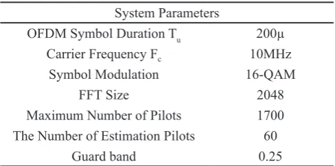
Table 1. System Parameters
System Parameters
OFDM Symbol Duration Tu 200µ Carrier Frequency Fc 10MHz
Symbol Modulation 16-QAM
FFT Size 2048
Maximum Number of Pilots 1700 The Number of Estimation Pilots 60
Guard band 0.25
In this section, we simulate the DVB-T2 system and investigate the impact of our proposed method on the estimated channel and performance of the system. We change the OFDM block of DVB-T2 system to prepare it for utilizing the sparse representation. Table 1 contains parameters of the simulated system indicated in fig.1. In this simulation, we have run the system a thousand times for each experiment and we have considered the mean of simulation results as the final result. In this simulation, we utilize sparse methods such as weighted SL0, W-SL0, and SL0 [22], as two methods of finding spare answer of P0 problem and weighted P0 problem, respectively. Besides these two methods, other methods such as l1-minimization [23] and LASSO [29] are used to find the sparse answer. We also have run the simulation for different signal to noise ratio (SNR) and different number of estimation pilots. Figures 2 and 3 illustrate the impact of contribution of side information on the channel estimation process. These figures plot Bit Error Rate (BER) of simulated
OFDM system versus different SNR while the numbers of estimation-pilots are fixed. As indicated, utilizing side information improves the performance of the system. To interpret this improvement, the assigned cost matrix which is correlated to side information that increases the cost of wrong answers. As illustrated at these figures 2 and 3, at the low SNR, by utilizing side information and improving the estimation channel, the performance of system is improved. However, at the high SNR the improvement ratio is reduced.
Utilizing side information provides the opportunities to release system resources such as the number of estimation-pilots assigned for estimating the channel. Figures 4 and 5 present the BER of system versus the number of estimated-pilots. These figures indicate improvements in the performance of system while fewer resources and side information are employed. These figures present that weighted-sparse algorithms result in better performance in compare with sparse algorithms at the same conditions. This reduction in occupying resources provides an opportunity to assign them for transmitting data and increasing capacity of data transmission. It also indicates that by utilizing side information, same performance could be achieved while fewer resources are employed.
6- Conclusion
In this paper, we introduce an approach to improve the results of OFDM sparse channel estimation. In this approach, some information about channel condition is extracted by employing previous estimation and coherence time of the channel. This information is employed to improve the estimation of the channel. In this regard, we define a diagonal cost matrix in correspondence with this information to
Fig. 3. Impact of channel Side Information on BER of OFDM system, WSL0-algorithm
convey side information into channel estimation process and provided weighted-dictionary. We also show that by replacing weighted dictionary and modifying sparse representation, ordinary sparse recovery algorithms become applicable to find the sparse answer. Furthermore, it is shown that utilizing side information not only increases the performance of the answer, but also releases the resources of the system.
Reference
[1] E.S. EN, 302 304: Digital Video Broadcasting (DVB), Transmission system for handheld terminals (DVB-H), ETSI, (2004).
[2] J.S. Proakis, M. Nov, 6, 2007” Digital Communications, in, McGraw-Hill Education.
[3] A. Goldsmith, Wireless communications, Cambridge university press, 2005.
[4] T. ETSI, 102 428: Digital Audio Broadcasting (DAB), DMB video service, (2009).
[5] O. Edfors, M. Sandell, J.-J. Van de Beek, S.K. Wilson, P.O. Borjesson, OFDM channel estimation by singular value decomposition, IEEE Transactions on communications, 46(7) (1998) 931-939.
[6] S. Coleri, M. Ergen, A. Puri, A. Bahai, Channel estimation techniques based on pilot arrangement in
OFDM systems, IEEE Transactions on broadcasting, 48(3) (2002) 223-229.
[7] H. Minn, V.K. Bhargava, An investigation into time-domain approach for OFDM channel estimation, IEEE Transactions on broadcasting, 46(4) (2000) 240-248.
[8] J.-J. Van De Beek, O. Edfors, M. Sandell, S.K. Wilson, P.O. Borjesson, On channel estimation in OFDM systems, in: Vehicular Technology Conference, 1995 IEEE 45th, IEEE, 1995, pp. 815-819.
[9] Y. Li, L.J. Cimini, N.R. Sollenberger, Robust channel estimation for OFDM systems with rapid dispersive fading channels, IEEE Transactions on communications, 46(7) (1998) 902-915.
[10] A. Petropulu, R. Zhang, R. Lin, Blind OFDM channel
estimation through simple linear precoding, IEEE Transactions on Wireless Communications, 3(2) (2004) 647-655.
[11] J.K. Tugnait, L. Tong, Single-user channel estimation and equalization, IEEE Signal Processing Magazine, 17(3) (2000) 17-28.
[12] P. Hoeher, S. Kaiser, P. Robertson, Two-dimensional
pilot-symbol-aided channel estimation by Wiener filtering, in: Acoustics, Speech, and Signal Processing, 1997. ICASSP-97., 1997 IEEE International Conference on, IEEE, 1997, pp. 1845-1848.
[13] P. Hoeher, S. Kaiser, P. Robertson, Pilot-symbol-aided channel estimation in time and frequency, Multi-carrier spread-spectrum, (1997) 169-178.
[14] M. Sandell, Design and analysis of estimators for
multicarrier modulation and ultrasonic imaging, Luleå tekniska universitet, 1996.
[15] M. Necker, F. Sanzi, J. Speidel, An adaptive
wiener-filter for improved channel estimation in mobile OFDM-systems, in: Proc. IEEE Intern. Symp. on Signal Proc. and Inf. Tech.(ISSPIT), 2001, pp. 213-216.
[16] X. Hou, S. Li, D. Liu, C. Yin, G. Yue, On
two-dimensional adaptive channel estimation in OFDM systems, in: Vehicular Technology Conference, 2004. VTC2004-Fall. 2004 IEEE 60th, IEEE, 2004, pp. 498-502
[17] S. Haykin, B. Widrow, Least-mean-square adaptive
filters, John Wiley & Sons, 2003.
[18] S. Haykin, B. Widrow, Least-mean-square adaptive
filters, John Wiley & Sons, 2003.
[19] S. Haykin, B. Widrow, Least-mean-square adaptive
filters, John Wiley & Sons, 2003.
[20] P. Pakrooh, A. Amini, F. Marvasti, OFDM pilot
allocation for sparse channel estimation, EURASIP Journal on Advances in Signal Processing, 2012(1) (2012) 59.
[21] C. Qi, L. Wu, A study of deterministic pilot allocation for sparse channel estimation in OFDM systems, IEEE communications letters, 16(5) (2012) 742-744.
[22] F. Wan, W.-P. Zhu, M. Swamy, Semi-blind most
significant tap detection for sparse channel estimation of OFDM systems, IEEE Transactions on Circuits and Systems I: Regular Papers, 57(3) (2010) 703-713.
[23] M. Elad, From Exact to Approximate Solutions, in:
Fig. 5. Impact of Side Information on Channel Estimation, Fixed SNR, WSL0 v.s. SL0
Sparse and Redundant Representations, Springer, 2010, pp. 79-109.
[24] E.J. Candes, J.K. Romberg, T. Tao, Stable signal
recovery from incomplete and inaccurate measurements, Communications on pure and applied mathematics, 59(8) (2006) 1207-1223.
[25] S.G. Mallat, Z. Zhang, Matching pursuits with
time-frequency dictionaries, IEEE Transactions on signal processing, 41(12) (1993) 3397-3415
[26] J.A. Tropp, Greed is good: Algorithmic results for
sparse approximation, IEEE Transactions on Information theory, 50(10) (2004) 2231-2242.
[27] G.H. Mohimani, M. Babaie-Zadeh, C. Jutten, Fast
sparse representation based on smoothed ℓ0 norm, in:
International Conference on Independent Component Analysis and Signal Separation, Springer, 2007, pp. 389-396.
[28] M. Elad, Sparse and Redundant Representations: From
Theory to Applications in Signal and Image Processing, Springer New York, 2011.
[29] Y. Nan, L. Zhang, X. Sun, An efficient downlink channel estimation approach for TDD massive MIMO systems,
in: Vehicular Technology Conference (VTC Spring), 2016 IEEE 83rd, IEEE, 2016, pp. 1-5.
[30] I.F. Gorodnitsky, B.D. Rao, Sparse signal reconstruction from limited data using FOCUSS: A re-weighted minimum norm algorithm, IEEE Transactions on signal processing, 45(3) (1997) 600-616.
[31] S.S. Chen, D.L. Donoho, M.A. Saunders, Atomic
decomposition by basis pursuit, SIAM review, 43(1) (2001) 129-159.
[32] J.O. Berger, Statistical Decision Theory and Bayesian Analysis, Springer, 1985.
[33] M. Unser, P.D. Tafti, An Introduction to Sparse
Stochastic Processes, Cambridge University Press, 2014.
[34] A. Papoulis, Probability & Statistics, Prentice Hall, 1990.
[35] R. Tibshirani, Regression shrinkage and selection via the lasso, Journal of the Royal Statistical Society. Series B (Methodological), (1996) 267-288.
[36] M. Babaie-Zadeh, B. Mehrdad, G.B. Giannakis,
Weighted sparse signal decomposition, in: Acoustics, Speech and Signal Processing (ICASSP), 2012 IEEE International Conference on, IEEE, 2012, pp. 3425-3428.
Pleasecitethisarticleusing:
S. Ghazi-Maghrebi, S. H. HashemiRafsanjani, Improved Channel Estimation for DVB-T2 Systems by Utilizing Side Information on OFDM Sparse Channel Estimation, AUT J. Elec. Eng., 50(3) (2018) 129-134.