A Non-radial rough DEA model

1

Available online at http://ijdea.srbiau.ac.ir

Int. J. Data Envelopment Analysis (ISSN 2345-458X) Vol. 1, No. 1, Year 2013 Article ID IJDEA-00111, 6 pages

Research Article

A Non-radial rough DEA model

G. Tohidi a, P. Valizadeha*

(a) Department of Mathematics, Islamic Azad University, Central Tehran Branch, Tehran - Iran

Abstract

For efficiency evaluation of some of the Decision Making Units that have uncertain information, Rough Data Envelopment Analysis technique is used, which is derived from rough set theorem and Data Envelopment Analysis (DEA). In some situations rough data alter nonradially. To this end, this paper proposes additive rough–DEA model and illustrates the proposed model by a numerical example.

Keywords: Rough data envelopment analysis (RDEA), Data envelopment analysis (DEA),

Uncertainty

1 Introduction

Data envelopment analysis (DEA), was first put forward by Charnes, Cooper and Rhodes (CCR model) in 1978 [1], it is performance measurement technique which can be used for evaluating the relative efficiency of Decision Making Units (DMU’s) in organizations.

One of research of DEA is Rough-DEA that researches on Rough-DEA (RDEA) are still very restricted. Therefore, the research on combining DEA with Rough set theory is an attractive study field.

Pawlak introduced a theory of Rough sets in 1982. Since then rough-set theory has been developed very rapidly and has resulted in a number of applications.

In order to provide an axiomatic theory to describe rough events, Liu [2], established the thrust theory which is branch of mathematics that studies the behavior of rough events.

Liu [2], defined a rough variable by a measurable function from a rough space (μ, ∆, Λ, π) to the

set of real numbers, that is for any Borel set B of R, Λ hold – Based on the thrust

theory, Liu and Jiuping Xu, bin Liu, Desheng Wu [2,3], studied some rough programming models with variables as parameters. The remainder of this paper is organized as follows.

In section 2 we want to bring some concepts about measurable space, Rough space and trust measure.

In section 3 we present the Additive Rough DEA (ARDEA) model, section 4 provides an application example to illustrate the efficiency of the ARDEA model. Finally, concluding remarks are outlined in section 5.

2 Background

* _{Corresponding author, Email address: [email protected].}



 





;







B





This section recalls several concepts of rough variable theory to characterize the rough uncertainty.

Definition 2.1[2]: Let μ be a nonempty sets, a collection Λ is called a – algebra of subsets of μ if is

satisfied in the following conditions: (a) μ Λ

(b) If A Λ, then Ac _Λ

(c) If Ai Λ, for i = 1… then

Definition 2.2[2]: Let μ be a nonempty set, and Λ a – algebra of subsets of μ, then (μ, Λ) is culled

a measurable space and the elements in Λ are called measurable sets furthermore, if π is measure defined on (μ, Λ), then triplet (π, Λ, π) is called measure space.

Definition 2.3[2]: Let μ be a nonempty set, Λ a – algebra of subsets of μ, ∆ an element in Λ, and π a set function on Λ, then (μ, ∆, Λ, π) is called rough space, furthermore, the triplet (μ, Λ, π) is a measure space.

Definition 2.4[2]: Uncertain variables: An uncertain variable is a measurable function from an uncertainty space (μ, Λ, π) to the set of real numbers, i.e., for any Borel set B of real numbers, the set

is an event.

Example [1]: Random variables, fuzzy variables and hybrid variable are instance of uncertain variable.

Definition 2.5[2]: Uncertain vector: An n-dimensional uncertain vector is a measurable function from

an uncertainly space (μ, A, π) to the set of n-dimensional real vectors, i.e., for any Borel set B of Rn,

the is an event.

Definition 2.6[2]: Let (μ, ∆, A, π) be a rough space then the upper trust of event A A is defined by .

The lower trust of the event A is defined by and the trust of the event A is defined

by Tr{A} = ½ ( + ).

Definition 2.7[2]: Let be a rough variable, and α (0, 1], then

is called the α – optimistic value to and is called the α –

pessimistic value to .

It is important to have focus that be a rough variable with then the

α – optimistic value of is

And the α – pessimistic value of is





 

 A A

i i  



1











B

















 





B









B













|



 



B





   

 







A A

T_r 

 





 

  





A

A Tr

 

A

T_r T

 

A

r







_sup

 



sup



r|Tr





r













_inf

 





inf



r

|

Tr







r











   



a,b, c,d







c



a



b



d

Theorem 1. [2]. Let and be the α-pessimistic and α-optimistic values of the rough

variable , respectively – then we have

(a) And

(b) is an increasing and left-continuous function of α;

(c) is a decreasing ad left-continuous function of α;

(d) If 0 < α ≤ 1, then = (1-α), and =

(e) If 0 < α ≤ 0.5, then ≤ ;

(f) If 0.5 < α ≤ 1, then ≤ ;

Definition 2.7[3]: Dmuo is rough DEA efficient if its best possible upper bound efficiency (ɵ*) inf (α)

Is equal to One; otherwise, it is said to be rough DEA inefficient if (ɵ*) inf (α) _<1.

3 Additive rough DEA

Let there are n DMUs and each DMU has m inputs and s outputs, the input and output vectors of

DMUj are rough vectors i.e.

According to the Additive DEA model (the following model), we can formulate a DEA model with rough.

Max

(1)

S-≥, S+≥0

Generally, to deal with the rough uncertainty discussed above , Liu [2], proposed the rough expected value model(EVM) and α – optimistic value and α – pessimistic value operator of rough variable to transfer rough programming in to determinate one.

 











 









 









                               otherwise c d a b c d a b c d a a b c c d c d b if d c c d c a if d c ) ( ) ( 2 2 2 1 2 1 2 2 2 2 1 inf



















 





inf



sup

 





 









_sup









Tr

Tr









 







a

;

 





inf

 





_sup

 





inf



sup

 





sup

 





inf



1







 





_inf



sup

 



 





inf



sup

 



n j y y y and x x

xj ij,... mj 0 _{i ij},..., _sj0 1,....,

                          





    m i s r Sr Si 1 1 . 0 ,..., 1 ,...., 1 . . 1 1           





j ro r n j rj j io i n j ij j s r y S y m i x S x t s







In this paper we suppose 0.5 < α ≤1, according to the theorem, α –value of the rough variable are

and and , it is denoted by .

3.1 Transfer rough model into deterministic model

Jiuping Xu,bin Liu,Desheng Wu[3],transferred the rough variables in model (1) into an interval

programming under trust level α, therefore rough variables 0 and

0 can be transformed to and .

And with assumption 0.5<α≤1 we have Now RDEA model (1) can be transformed

in to following program:

Max

.

In order to transform the interval programming (2) in to deterministic linear programming with α trust level we assume:

DMUo max output

DMUj min output j o

Now interval programming (2) can be transformed in to programming (3) as following

Si- ≥0 i=1,…,m , Sr+≥0 r=1,…,s , j=1,…., n.

The variables in the model (3) are not rough, i.e. they are deterministic, and the model (3) is a linear

program. In model (3) DMUo is ARDEA-efficient if and only if S-* =0 and S+*=0.



 





sup



inf

 





inf

 







sup

 







sup

 



,



inf

 





           t mj ij

j x x

x ....            t mj ij

j y y

y ....



sup  int 



, _j

j x

x



ysup_j   ,yint_j  



 

_sup

 

.

inf











 

2

1 1       





    m i s r r i S S    







   



m i x x x x t

s _{io io}

n

j

ij ij

j , , 1,...,

. sup inf

1

inf

sup _{ }



    



   







   



s r y y y

y ro ro

n

j

rj rj

j , , 1,...,

inf sup

1

inf

sup _{ }



    



. ,..., 1 ,

0 j n

j  



inputs min outputs max 

 

3 max 1 1       





    s r r m i i S S       m i x S x x t

s _{jo jo i io}

n

j ij

j 1,...,

. sup sup

inf 1      



_  _         s r y S y

y_{rj io ro r ro}

j 1,...,

inf inf

sup _{ }  _{ }



_  _  

0 

j

4 Practical application

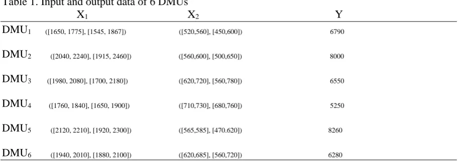
In this section, we will evaluate the operation performance of the six DMUs with two inputs and one output (see Table 1) using the proposed ARDEA model.

Table 1. Input and output data of 6 DMUs

X1 X2 Y

DMU1 ([1650, 1775], [1545, 1867]) ([520,560], [450,600]) 6790

DMU2 ([2040, 2240], [1915, 2460]) ([560,600], [500,650]) 8000

DMU3 ([1980, 2080], [1700, 2180]) ([620,720], [560,780]) 6550

DMU4 ([1760, 1840], [1650, 1900]) ([710,730], [680,760]) 5250

DMU5 ([2120, 2210], [1920, 2300]) ([565,585], [470.620]) 8260

DMU6 ([1940, 2010], [1880, 2100]) ([620,685], [560,720]) 6280

4.2 Performance evaluation

Using the transformation technique described in the previous section, we transform the rough variables in Table 1 into certain variables. Suppose the trust level α=0.9, the corresponding programming model’s solutions of DMUs are summarized in table2:

Table 2. The result for ARDEA model

DMU DMU1 DMU2 DMU3 DMU4 DMU5 DMU6

ARDEA model 0.00 432.88 0.00 0.00 788.10 0.00

In Table 2, DMU1, DMU3, DMU4 and DMU6 are ARDEA-efficient, i.e. the summations of their

slacks are zero.

5. Conclusion

In this paper, we have developed an ARDEA model with rough parameters. This model can be used to evaluate the performance of DMUs when they want to change their inputs and outputs non-redially. In the process of solving the ARDEA model, we used the α–optimistic value and α–pessimistic value of rough variable to transfer the rough model into deterministic liner programming. Finally we illustrate the proposed method by an example.

References

[1] A.Charnes, W.W.Cooper and E.Rhodes, 1978.Measurment the efficiency of decision making

units, Eur.J.Oper.Res.2, 429-444.

[2] Liu, B.D., 2004.Uncertain Theory: An Introduction to its Axiomatic Foundation. Springer,

Berlin.

[3] Jiuping Xu, Bin Li, Desheng Wu, 2009. Rough data envelopment analysis and its application