Optimal Power Flow With Four Conflicting Objective Functions Using Multiobjective Ant Lion Algorithm: A Case Study of the Algerian Electrical Network

(1)

Iranian Journal of Electrical and Electronic Engineering, Vol. 15, No. 1, March 2019 94

Optimal Power Flow With Four Conflicting Objective

Functions Using Multiobjective Ant Lion Algorithm: A Case

Study of the Algerian Electrical Network

O. Herbadji*, L. Slimani* and T. Bouktir*

(C.A.)

Abstract: In this study, a multiobjective optimization is applied to Optimal Power Flow Problem (OPF). To effectively achieve this goal, a Multiobjective Ant Lion algorithm (MOALO) is proposed to find the Pareto optimal front for the multiobjective OPF. The aim of this work is to reach good solutions of Active and Reactive OPF problem by optimizing 4-conflicting objective functions simultaneously. Here are generation cost, environmental pollution emission, active power losses, and voltage deviation. The performance of the proposed MOALO algorithm has been tested on various electrical power systems with different sizes such as IEEE 30-bus, IEEE 57-bus, IEEE 118-bus, IEEE 300-bus systems and on practical Algerian DZ114-bus system. The results of the tests proved the versatility of the algorithm when applied to large systems. The effectiveness of the proposed method has been confirmed by comparing the results obtained with those obtained by other algorithms given in the literature for the same test systems.

Keywords: Optimal Power Flow, Multiobjective Ant Lion Algorithm, Algerian Electrical

Network, Generation Cost, Environmental Pollution Emission, Active Power Losses, Voltage Deviation.

1 Introduction1

PTIMAL Power Flow (OPF) is one of the tasks in power system planning that helps the operators to run the system optimally under specific constraints. It has been extensively investigated since the pioneering work of Carpentier [1] in 1962. OPF can be applied periodically to minimize the total thermal unit fuel cost, emission of particulate and gaseous pollutants, real power loss, and to enhance voltage stability and to improve voltage profile as well. These can be achieved while satisfying certain constraints imposed by the network.

The OPF problem has been developed through the years from a single-objective optimization problem into a multiobjective optimization problem. Several methods

Iranian Journal of Electrical and Electronic Engineering, 2019. Paper first received 25 June 2018 and accepted 26 November 2018. * The authors are with the Department of Electrical Engineering, Université Ferhat Abbes Setif 1, Setif, Algeria.

E-mails: [email protected], [email protected] and [email protected].

Corresponding Author: T. Bouktir.

have been developed to solve multiobjective optimization problems. For example, the method of the penalty function [2] and the weighted sum method [3] have been used to solve various multiobjective optimization problems. However, these methods have shortcomings and face difficulties. For example the penalty function method, choosing the appropriate penalty factors is a difficult task and it is too sensitive to the associated penalty parameters [4]. The weighted sum approach combines all the objectives with one goal using weighting factors. This formulation may lose the importance of the objective function and there is no a rational basis for determines the weighting factors of the non-commensurable objectives [5]. In order to overcome the drawbacks of these optimization methods, a wide variety of global optimization techniques have been developed to solve OPF in such complex power systems. These techniques are based on heuristic and stochastic aspects such as; Genetic algorithm (GA) [6-8], Particle Swarm Optimization (PSO) [9], Differential evolution (DE) [10], Artificial bee colony (ABC) [11], Biogeography based optimization method (BBO) [12, 13], Gravitational search algorithm (GSA)

O

(2)

[14], Black hole algorithm (BH) [15],Cuckoo Optimization Algorithm (COA) [14], Grey Wolf Optimization (GWO) ,Ant Lion Optimization (ALO), Crow Search Algorithm (CSA), Dragonfly Algorithm (DA) [16].

Because of the nature of multiobjective problems, relational arithmetic operators cannot perform the comparison between different solutions. The concepts of Pareto optimal dominance allow us to compare multi-solutions in a multiobjective search space. There is no best solution, but a preferable solution. This means that several solutions are calculated, with different trade-offs between conflicting objectives and the engineer will select among them the most preferable for the problem at hand [17].

The OPF is an example of multiobjective optimization problems involving two, three objectives and in practically; the OPF can have more than three objectives [18-21].

In [18], authors proposed the use of multiobjective modified imperialist competitive algorithm (MOMICA) for the OPF problem which is applied to IEEE 30-bus and 57-bus test systems in order to solve four conflicting functions, generation cost, environmental pollution, voltage magnitude deviations and power losses.

In [19], Artificial bee colony algorithm with dynamic population (ABCDP) is proposed to solve multi-optimal power flow problems in power systems that consider the fuel cost, power losses, and emission impacts as objective functions.

Authors in [20] proposed two novel Jaya-based algorithms for solving different MOOPF problems; the modified Jaya algorithm (MJaya) and quasi-oppositional modified Jaya algorithm (QOMJaya). In this study the objectives functions were the fuel cost and the gas emission.

In [21], we proposed the use of multiobjective Dragonfly algorithm to solve single-objective, discrete, and multiobjective problems. The objectives were to reduce the total generation fuel cost, environmental pollution caused by fossil-based thermal generating units, active power losses and the voltage deviation. In this paper a multiobjective optimization of optimal power flow (MOOPF) is carried out by using one of the latest meta-heuristic optimization techniques; the multiobjective ant lion algorithm (MOALO) using elitist non-dominating solution. MOALO technique is a new bio-inspired algorithm developed by Seyedali Mirjalili in 2016 [22], inspired from the behavior of ant lion to hunt a prey in nature.

The developed MOALO-based algorithm is applied and tested on the IEEE 30-bus, IEEE 57-bus, IEEE 118-bus systems and the Algerian electrical network DZ 114-bus for six cases of MOOPF problems. Fuel cost, total gas emission, total active losses and voltage deviation were considered to be the objective functions to be optimized. The Obtained results are compared

with those of algorithms given in the literature for the same test systems to prove the effectiveness and the superiority of the proposed algorithm [21-23].

The remainder of this paper is organized as follows; in Section 2, the MOOPF problem is mathematically formulated. Then, the details of the proposed method are discussed. Next, we apply the proposed MOALO approach to solve the multiobjective OPF problem. Simulation results are presented and discussed in Section 5. Finally, Section 6 concludes the paper.

2 Problem Formulation

The task of multiobjective optimization is to find solutions to problems with several objective functions to optimize [25]. Multiobjective problem can be formulated as follows:

 



 



1 2 3

Minimize , , , ,

nobj

F x f x f x f x

f x

 

(1) Subject to:

 

0, 1, 2, 3, ,

i

g x  i  m (2)

 

0, 1, 2, 3, ,

i

h x  i   p (3)

, 1, 2, 3, ,

i i i

L x U i  n (4)

wheref₁

 

x , f₂

   

x , f₃ x , are the objective functions, x is the vector of control variables, gi and hi

are the i-th inequality and equality constraints respectively, n is the number of variables, nobj is the number of objective functions, m and p are the numbers of equality and inequality constraints respectively and Li, Ui are the limits of i-th variable.

The MOOPF is formulated as to minimize simultaneously different objective functions namely; the total fuel cost, the total emission, the active power losses and the voltage deviation.

2.1 Total Fuel Cost Function

The total fuel cost of production (F1) of the real power of the interconnected generators is given by the quadratic function [26, 27].

 



2



1

1 ng

i i gi i gi

i

F x A B P C P





  (5)

where Ai, Bi and Ci are the fuel cost coefficients of the

generating unit i, Pgi is the generated active power at

bus i and ng is number of generators including the slack bus.

2.2 Total Emission Function

The objective function (F2) for emission minimization can be expressed as a combination of quadratic and exponential functions of the generated active power [28]:

(3)

 



2





2

1

exp

ng

i i gi i gi i i gi

i

F x a b P c P d e P





   (6)

where ai, bi, ci, di and ei are the total emission

coefficients.

2.3 Function of Active Power Losses

The minimization of real power losses in the transmission network is one of the important objectives of the OPF problem. The function of active power transmission losses (F3) is given by

 



2 2



3

1

2 n

loss K i j i j ij

i

F x P G V V V V cos



 



  (7)

where n is the branch number on the network, K is a branch with conductance G connecting the i-th bus to the j-th bus.

2.4 Voltage Magnitude Deviation Function

The objective is to minimize the voltage magnitude deviation at the load buses given by

 

4 1 1 Nbus M i

F x V V i



  



 (8)

where VMis the voltage in each bus of the network.

2.5 Minimization of the Voltage Stability Index (VSI)

The voltage stability index (VSI) is one of different indices for voltage stability and voltage collapse prediction. The voltage stability index can be defined as:

 





 





5 min max index L j

F x F x

V SI Min L    (9) with



1







1 2

1

1 [ ] [ ]

, 1, 2, , w N

i

j ij i j

i j

PQ

V

L Y Y

V j N           _      _    



(10)

where Y1 and Y2 are the sub-matrices of the Ybus and the

operating range of L was set between [0-1].

2.6 Equality and Inequality Constraints

The multiobjective OPF constraints can be split into two parts: equality and inequality constraints. Equality constraints are the active and reactive power balance equations (Eq. (11)).





1

cos sin

i i

g d i j ij ij ij ij

j N

P P V V g  z 

  









1 sin cos i i

g d i j ij

N

j

ij ij ij

Q Q V V g  z 



 



 (11)

The inequality constraints are presented as follows. – Generators limits:

min max

i i i

g g g

P P P

min max

i i i

g g g

Q Q Q

min max

i i i

g g g

V V V (12)

– Tap transformer limits:

min max

T  T T (13)

– Voltage magnitude for load buses limits:

min max

i i i

L L L

V V V (14)

– Power flow of transmission lines limits:

min max

i i i

L L L

S S S (15)

3 Multiobjective Antlion Optimizer (MOALO)

Antlion Optimizer (ALO) is a new nature-inspired algorithm proposed by Seyedali Mirjalili in 2016 [22] for solving constrained engineering optimization problems. ALO algorithm mimics the hunting mechanism of antlions in nature and the interaction of their favorite prey-ants- with them. The general steps of ALO which, describe the interaction between antlions and ants in the trap are as follows: Random walk of ants, building traps, entrapment of ants in traps, catching preys and rebuilding the traps and elitism. Fig. 1(a) represent one of the cone-shapeds pits building by the antlions. In Fig. 1(b) the predator (antlion) hide in the bottom of the pit and waiting his prey (ant) to catch it. After catching the prey, the antlion

(a)

(b)

Fig. 1 Interaction the last between the antlions and ants in the trap.

(4)

rebuilding the traps for the next hunt. The main inspiration of ALO method is that the predators tend to dig a big trap when they is hungry.

The original random walk used in the ALO algorithm to simulate the random walk of ants is expressed as follows:

 



 



 





 





1 2

0, 2 1 ,

2 1 , ,

2 _n 1

X t cumsum r t

cumsum r t



_ 

 



  (16)

where, cumsum determines the cumulative sum, n shows the maximum number of iteration, t presents the step of random walk (iterations), and r(t) is a stochastic function given as:

 

1 if 0.5

0 if 0.5 rand r t rand     _  (17)

where rand is a random number generated in the interval [0, 1].

To keep the random walk in the limits of the search space and prevent the ants from overshooting, the random walk is designated using the following expression:











t t t

i i i i

t t

i i

X a d c

X c

b a

 

 

 (18)

where d_it and c_it indicate the maximum and minimum of i-th variable at t-thiteration respectively, ai and bi are

the minimum and maximum of random walks corresponding to the i-th variable, respectively.

The model of the trapping mechanism of antlions on ants is expressed by the Eqs. (19) and (20):

t t t

i j

c Antlion c (19)

t t t

i j

d Antlion d (20)

where ct_and_dt_{are the minimum and the maximum of}

all variables at t-th iteration, ct_and_dt_{are the minimum}

and the maximum of all variables for i-th ant, and t

j

Antlion represents the position of the selected j-th antlion at t-thiteration.

In the nature, bigger pits are built by bigger antlions to increase their chance of survival. Mathematically this step is given below as:

t t c c I  (21) t t d d I  (22) where 10 max w t I iter

 is the maximum number of

iteration, t is the current iteration and w is a constant depends on t. w is defined as a follows:

2 when 0,1

3 when 0, 5

4 when 0, 75

5 when 0, 9

6 when 0, 95

t maxiter

w t maxiter

t maxiter t maxiter    _     _   

In ALO, the following equation simulates the catching of the ant and rebuilding the pit:



 



if :

t t t t

j j j j

Antlion Ant f Ant f Antlion (23)

where, t indicates the current iteration and t j

Ant shows the position of i-th ant at t-th iteration.

The last step in ALO is elitism; where the best antlion obtained is selected and stored as an elite during the optimization process. Since the elite is the fittest antlion, it is able to affect the movements of the remaining ants along the iterations. Therefore, the position update of every ant is depending on the random walks around a selected antlion by the roulette wheel and the elite. The elitism mechanism is explained by this equation:

2

t t

t A E

j

R R

Ant   (24)

where, t A

R is the random walks selected by the roulette wheel at t-th iteration around the antlion, and t

E R is the random walk at t-th iteration around the elite.

● Pareto Optimal Solution

The pareto optimal approach is an effective method for the multiobjective optimization problem. This method includes a group of dominant answers that make compromise between objective functions. The Pareto-optimal solutions are illustrated as a diagram named “Pareto diagram”. In the multiobjective optimization problem, any solution X1 is dominant or none dominant the other solution X2. Generally, X1 is assumed to dominate X2 only if two conditions are satisfied [29]:



1, 2, ,



: i

 

1 i

 

2

i n F X F X

   



1, 2, ,



: j

 

1 j

 

2

j n F X F X

    (25)

● Best Compromise Solution (BCS)

In the MOALO approach, the non-dominated solutions are saved in a repository in all iterations. These solutions are stored by the decision maker function (power system operator). To select the best solution from the Pareto optimal solution, we apply the roulette wheel method at each iteration to obtain a membership function. The membership function h

i

μ of

(5)

the i-thobjective function Fi is defined as [29]:

1

0

min

i i

max

h i i min max

i max min i i i

i i

max

i i

F F

F F F

F F



 

  

_  

 

 _



(26)

where, F_imin and F_imax represent the minimum and the maximum value of the i-th objective function Fi.

When Eq. (26) is a maximum, the best non-dominated solution is defined as follows:

1

1 1

obj

N _h

i

h i

M N _h

i

j i

 

 

 





 

(27)

where, M presents the number of the non-dominate solution.

●

MOALO utilizes an archive to store and retrieve the best approximations of the non-dominated Pareto optimal set during optimization. Then, the solutions are chosen from this archive by the mechanism of the roulette wheel based on the coverage of solutions as antlions to lead ants towards promising regions of multiobjective search spaces.

The details of the MOALO method are represented in Fig. 2 as a follows:

4 MOALO for Multiobjective Optimal Power Flow (MOOPF)

The computational procedure for solving the MOOPF problems using MOALO method is described in the following steps:

Step 1: Initialize the parameters of system, and specify the boundaries of all variables.

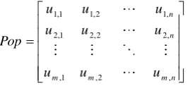
Step 2: Generate the initial population Pop based on the upper and lower limits of the control variables Eq. (25). The vector of control variable can be generated using active and reactive powers, bus voltage magnitudes, and transformers tap values, etc.

While the end condition is not met For every ant

Select a random antlion from the archive

Select the elite using roulette wheel from the archive Update ct_{and d}t_{using Eqs. (21) and (22)}

Create arandom walk and normalize it using Eqs. (16) and (18)

Update the position of the ant using Eq. (23) End for

Calculate the objective values for all ants Update the archive

End while Return archive

Fig. 2 Pseudo code of MOALO approach.

1,1 1,2 1,

2,1 2,2 2,

,1 ,2 ,

n

m m m n

u u u

Pop

u u u

 

 

_ _

 

 

(28)

The variable uk,j of the population can be described as

follows:









min max min

, , *

k j j j j

u u rand Np D u u (29)

where, Np is the number of search agents, D is the

dimension of the vector variable and umax_j and umin_j are the upper and lower limits of the j-th variable, respectively.

Step 3: Run the Newton Raphson load flow program to

calculate the objective functions and evaluate the particles in the population.

Step 4: Apply Pareto optimal method and store the

non-dominated solution.

Step 5: use the roulette wheel to choose a random solution from the archive and the elite, next, update parameters ct_and_dt_{by using Eqs. (21) and (22). After,}

create and normalize a random walk using Eqs. (12) and (18). Next, update the position of ant by Eq. (23). Step 6: Calculate the objective values of each ant and update the archive.

Step 7: Determine the non-dominated solutions using the Pareto method.

Step 8: If the current iteration number reaches the maximum iteration number stop and go to step 5. Step 9: Find the best compromise solution from the Pareto optimal solutions.

5 Case Studies

To verify the effectiveness of the proposed algorithm, different scales of power system cases have been considered: IEEE 30-bus, IEEE 57-bus, the IEEE 118-bus system and the Algerian transmission network DZ 114-bus (Fig. 3).

In these studies, six cases are discussed to demonstrate the usefulness of the proposed approach:

 Case 1: Fuel cost

 



1

 



Minimize F x  F x (30)

 Case 2: Fuel cost + Emission

 



1

 

2

 



Minimize F x  F x , F x (31)

 Case 3: Fuel cost + Real power losses

 



1

 

3

 



 Case 4: Fuel cost + Voltage magnitude deviation

 



1

 

4

 



(6)

Iranian Journal of Electrical and Electronic Engineering, Vol. 15, No. 1, March 2019 99 Fig. 3 Topology of the Algerian 114-bus power system [30].

 Case 5: Fuel cost + Emission + Power losses

 



1

 

2

 

3

 



Minimize F x  F x ,F x , F x (34)

 Case 6: Fuel cost + Emission + Power losses + Voltage magnitude deviation

 



1

 

2

 

3

 

4

 



Minimize F x  F x , F x , F x , F x (35)

The MOALO parameters utilized in this study is represented in Table.1.

5.1 IEEE 30-Bus Test System

The IEEE 30-bus test system [31, 32], comprises 6 generators installed at buses n° :1, 2, 5, 8, 11, and 13, forty one transmission lines including 4 transformers between buses (6-9), (6-10), (4-12), (28-27) and 9 compensators at the loads buses n° 10, 12, 15, 17, 20, 21, 23, 24, and 29 [33].The total load active power of this system is 2.834 pu at 100 MVA base.

The vector of control variables of IEEE 30-bus test system includes the generated active powers, magnitude voltages of generators, transformer tap settings and the capacitor banks.

2 5 8 11 13

g g g g g 1 2 5 8 11 13 6-9

6-10 4-12 28-27 c10 c12 c15 c17 c20 c21

c23 c24 c29

= [P ,P ,P ,P ,P ,V ,V ,V ,V ,V ,V ,T , T ,T ,T ,Q ,Q ,Q ,Q ,Q ,Q , Q ,Q ,Q ]

x

(36)

Table.1 Control parameter settings of MOALO algorithm for test systems.

Parameter Setting Value

Number of search agents (NSA) 100 Number of iterations 100 / 500

Archive maximum size 100

Search domain (rand) [0 1]

In this simulation, 100 test runs were carried out for solving multiobjective optimal power flow problem using the proposed algorithm. Table 2 represents the best result of the simulation obtained from the MOALO algorithm for six cases, Tables 3 and 4 present the comparison between the results obtained by MOALO-MOOPF and other multiobjective techniques for All cases.

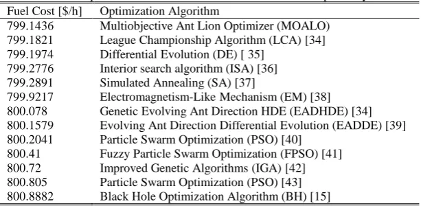
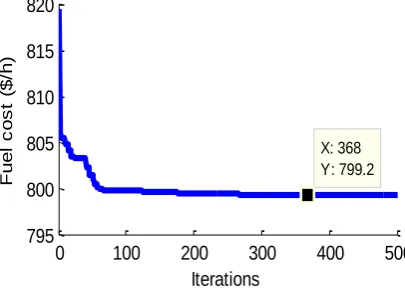
In the case 1, the only objective function is minimization of quadratic cost function. The BCS results in this case are presented in Table 2 and the convergence curve is exposed in Fig. 4. From Table 2 and Table 3; we can observe that the best compromise solutions obtained by MOALO as ($799.1436/h) is better than those obtained by the others methods. The results obtained from case 2 trough case 6 are also presented in Table 2, and the set of dominant points of these results is illustrated in Fig 5. Table 3 presents the comparison of the proposed MOALO with other heuristic methods previously cited in the literature. It is

(7)

Iranian Journal of Electrical and Electronic Engineering, Vol. 15, No. 1, March 2019 100 Table 2 Best results of multiobjective OPF problem for six cases using MOALO algorithm for IEEE 30-bus power

system.

Cases Min Case 01 Case 02 Case 03 Case 04 Case 05 Case 06 Max

Pg1 50 176.9100 121.9200 126.9200 178.7300 129.0300 130.9900 200

Pg2 20 48.7224 56.1451 54.1799 47.1804 53.9095 62.0566 80

Pg5 15 21.2700 33.4646 31.8519 20.6585 33.5281 26.6447 50

Pg8 10 21.2925 31.2523 29.0306 19.5493 25.9640 20.8269 35

Pg11 10 11.8465 23.6992 23.2661 13.5921 23.9419 24.5149 30

Pg13 12 12.0000 22.5619 23.9276 14.9793 23.1179 25.5783 40

Vg1 0.9 1.1000 1.0998 1.0995 1.0005 1.1000 1.0478 1.1

Vg2 0.9 1.0881 1.0921 1.0950 1.0054 1.1000 1.0540 1.1

Vg5 0.9 1.0620 1.0758 1.0801 1.0026 1.1000 1.0556 1.1

Vg8 0.9 1.0700 1.0826 1.0870 1.0183 1.1000 1.0455 1.1

Vg11 0.9 1.1000 1.0946 1.0884 1.0416 1.0936 1.0458 1.1

Vg13 0.9 1.1000 1.0785 1.0764 1.0070 1.0907 1.0594 1.1

T6-9 0.9 1.0066 1.0944 1.0865 0.9868 1.1000 1.0436 1.1

T6-10 0.9 0.9444 1.0871 1.0892 0.9380 1.1000 1.0576 1.1

T4-12 0.9 1.0095 1.0890 1.0855 0.9584 1.0896 1.0636 1.1

T28-27 0.9 0.9702 1.0947 1.0675 0.9568 1.0894 1.0108 1.1

Qc10 0 3.2615 2.4824 2.3749 2.4977 2.9352 3.3352 5

Qc12 0 4.6706 3.4092 2.8808 3.9472 3.5515 1.5559 5

Qc15 0 4.7018 2.6738 3.2391 3.2233 1.7035 2.1951 5

Qc17 0 4.1172 2.0257 2.4554 3.0011 2.5251 3.4373 5

Qc20 0 2.1428 1.1407 3.5667 2.3662 2.0506 3.5225 5

Qc21 0 1.7861 1.3482 1.9240 2.0403 3.4073 2.6896 5

Qc23 0 3.1086 2.7192 4.0104 1.8238 1.7189 3.2877 5

Qc24 0 4.5001 2.2566 3.8068 2.1653 2.0920 1.8451 5

Qc29 0 1.3933 1.3195 2.4957 3.1947 3.2858 2.9628 5

Fuel Cost [$/h] - 799.1436 831.6764 826.4556 803,0611 828.3344 826.2676 -

Emission [ton/h] - 0.3679 0.2576 0.2642 0.3718 0.2668 0.2730 -

Ploss [MW] - 8.6400 5.639 5.7727 11.2870 6.0932 7.2073 -

DV [pu] - 2.1930 1.2870 1.2560 0.0900 1.4080 0.7160 -

Table 3 Comparison of the BCS for cases 1 of IEEE 30-bus power system. Fuel Cost [$/h] Optimization Algorithm

799.1436 Multiobjective Ant Lion Optimizer (MOALO) 799.1821 League Championship Algorithm (LCA) [34] 799.1974 Differential Evolution (DE) [ 35]

799.2776 Interior search algorithm (ISA) [36] 799.2891 Simulated Annealing (SA) [37]

799.9217 Electromagnetism-Like Mechanism (EM) [38] 800.078 Genetic Evolving Ant Direction HDE (EADHDE) [34] 800.1579 Evolving Ant Direction Differential Evolution (EADDE) [39] 800.2041 Particle Swarm Optimization (PSO) [40]

800.41 Fuzzy Particle Swarm Optimization (FPSO) [41] 800.72 Improved Genetic Algorithms (IGA) [42] 800.805 Particle Swarm Optimization (PSO) [43] 800.8882 Black Hole Optimization Algorithm (BH) [15]

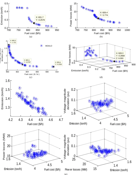
clear that the application of MOALO method to the multiobjective optimal power flow is giving better solutions than other algorithms and the Pareto optimal solutions are diverse and good distributed over the Pareto front. For example, in case 6 MOALO provides a minimum fuel cost and minimum voltage magnitude deviation compared with four recent algorithms ($826.2676/h and 0.0189 pu).

5.2 IEEE 57-Bus Test System

IEEE 57-bus test system constitutes of 7 generators,

80 transmission lines, 17 transformers and three capacitor banks [18]. The limits of voltage buses and transformer tap settings are between 0.9 and 1.1 pu [36]. The vector of control variables in this case also includes the generated active powers, magnitude voltages of generators, transformer tap settings and the capacitor banks’ sizes.

Results of simulation obtained from the proposed method of all cases are presented in Table 5. A comparison for case 1 and for the rest of cases is cited in Table 6 and Table 7, respectively.

(8)

Iranian Journal of Electrical and Electronic Engineering, Vol. 15, No. 1, March 2019 101 Table 4 Comparison of the BCS for case 2 through 6 of IEEE 30-bus power system.

Case 2: Fuel Cost +Emission

Fuel Cost [$/h] Emission [ton/h] Ploss [MW] DV [pu]

MOALO 831.6764 0.2576 - -

MOMICA[9] 865.0660 0.2221 - -

BB-MPSO[9] 865.0985 0.2227 -

Case 3 : Fuel Cost +Ploss

MOALO 826.4556 - 5.7727 -

MJaya[20] 826.9651 - 5.7596 -

QOMJaya[20] 827.9124 - 5.7960 -

MOABC/D[44] 827.6360 - 5.2451 -

NKEA[20] 829.4911 - 5.8603 -

MOMICA[9] 848.0544 - 4.5603 -

MODA[10] 842.7550 - 5.2090 -

Case 4 : Fuel Cost +DV

MOALO 803,0611 - - 0,3787

MODA[10] 804.6862 - - 0.0114

MOMICA[9] 804.9611 - - 0.0952

BB-MPSO[9] 804.9639 - - 0.1021

MINSGA-II[9] 805.0076 - - 0.0989

ISA[36] 807.6408 - - 0.1273

Case 5 : Fuel Cost +Emission +Ploss

MOALO 828.3344 0.2668 6.0932 -

MODA[10] 867.9070 0.2640 5.9110 -

Case 6 : Fuel Cost +Emission +Ploss +DV

MOALO 826.2676 0.2730 7.2073 0.0189

MODA[10] 828.4912 0.2648 5.9119 0.0585

MOMICA[9] 830.1884 0.2523 5.5851 0.2978

BB-MPSO[9] 833.0345 0.2479 5.6504 0.3945

NKEA[20] 834.6433 0.2491 5.8935 0.4448

0 100 200 300 400 500

795 800 805 810 815 820

X: 368 Y: 799.2

Iterations

Fu

e

l

c

o

s

t

($

/h

)

Fig. 4 The convergence of MOALO algorithm for IEEE 30-bus system in case 1.

In this simulation, Table 5 shows the best values of four competing objectives optimized by the MOALO. Convergence diagram of the fuel cost (case 1) is shown in Fig. 6 and the Pareto-optimal results from case 2 to case 6 are illustrated in Fig. 7. The comparison shown in Tables 6 and 7 prove that MOALO gives better results

except in the last case where the power losses and the fuel cost are lower than those obtained by NKEA method by a percentage of -1.76% and -19.85%, respectively, but the emission and the voltage deviation are better by 5.84% and 92.04%, respectively. As a conclusion, MOALO is better than KNEA.

(9)

700 750 800 850 900 950

0.2 0.3 0.4 0.5 X: 831.7 Y: 0.2576

Fuel cost ($/h)

E m is s io n ( to n /h )

700 750 800 850 900 950 1000

0 5 10 15 X: 826.4 Y: 5.774

Fuel cost ($/h)

P o w e r lo s s e s ( M W ) (a) (b)

800 802 804 806 808 810

0 0.5 1 1.5 2 X: 803.1 Y: 0.3787

Fuel cost ( $ / hr )

V o lt a g e m a g n it u d e d e v ia ti o n ( p u ) X: 809.4 Y: 0.2353 X: 800.3 Y: 1.721 MOALO 700 750 800 850 900 0.2 0.3 0.4 0.50 50 X: 828.3 Y: 0.2668 Z: 6.093

Fuel cost ($/h) Emission (ton/h) P o w e r lo s s e s ( M W ) (c) (d)

4

4.5

5

1.4

1.6

0

0.1

0.2

Fuel cost ($/h)

Emission (ton/h)

V o lt a g e m a g n it u d e d e v ia ti o n ( p u )

1.4

1.6

15

20

25

0

0.1

0.2

Emission (ton/h)

Pow er losses (MW)

V o lt a g e m a g n it u d e d e v ia ti o n ( p u )

4

4.5

5

1.4

1.6

15

20

25

Fuel cost ($/h)

Emission (ton/h)

P o w e r lo s s e s ( M W )

4.2

4.3

4.4

4.5

4.6

4.7

1.3

1.4

1.5

1.6

Fuel cost ($/h)

E m is s io n ( to n /h ) (e)

Fig. 5 Pareto-optimal solutions obtained in cases 2 through 6 for best solution for IEEE 30-bus power system; a) Case 02– Fuel cost + Emission, b) Case 03– Fuel cost +Ploss, c) Case 04– Fuel cost + DV, d) Case 05– Fuel cost +Emission +Ploss, and e) Case 06–

Fuel cost + Emission +Ploss +DV.

(10)

Iranian Journal of Electrical and Electronic Engineering, Vol. 15, No. 1, March 2019 103 Table 5 Results of MO-OPF problem for 6-cases using MOALO algorithm of 57-bus test system.

Cases Case 01 Case 02 Case 03 Case 04 Case 05 Case 06

Pg1 396.9100 214.3100 148.2700 156.3800 231.7600 207.7700

Pg2 119.5583 98.7031 68.4795 97.5843 19.0593 68.1618

Pg3 92.0553 98.5652 53.7031 49.4052 66.7253 80.1569

Pg6 43.8150 84.0391 99.7128 36.2118 92.0849 96.8831

Pg8 89.2414 383.0225 424.5749 479.7535 345.8168 337.1985

Pg9 453.6108 100.0000 99.2418 92.5269 99.7837 98.8692

Pg12 94.3669 292.6367 375.0308 365.9775 409.7688 377.2544

Vg1 1.0973 1.0107 1.0988 1.0241 1.1000 1.0153

Vg2 1.0999 0.9616 1.0971 1.0238 1.1000 1.0136

Vg3 1.0901 0.9633 1.0893 1.0116 1.1000 1.0043

Vg6 1.0986 0.9378 1.0899 1.0096 1.0913 0.9996

Vg8 1.1000 1.1000 1.1000 1.0360 1.1000 1.0184

Vg9 1.0962 0.9539 1.1000 1.0238 1.0910 1.0214

Vg12 1.0849 0.9423 1.0957 1.0122 1.0999 1.0165

T4-18 1.0865 0.9608 1.0987 1.0166 0.9940 1.0157

T4-18 1.0799 0.9736 1.1000 1.0104 1.1000 0.9937

T21-20 1.0942 0.9553 1.1000 0.9762 1.1000 1.0031

T24-25 1.0489 1.0883 1.0963 1.0224 1.0000 1.0048

T24-25 1.0661 0.9703 1.1000 0.9887 0.9912 1.0120

T24-26 1.0535 0.9524 1.0921 1.0368 0.9928 1.0130

T7-29 1.0428 1.0984 1.0958 0.9811 0.9999 0.9847

T34-32 0.9861 1.0970 1.1000 0.9679 0.9963 1.0279

T11-41 1.0400 1.0984 1.1000 0.9813 1.1000 1.0096

T15-45 1.0160 1.1000 1.0971 0.9521 1.1000 0.9952

T14-46 1.0108 1.0996 1.0969 0.9544 1.0959 0.9803

T10-51 1.0261 1.1000 1.0867 0.9628 1.0972 0.9826

T13-49 0.9867 0.9742 1.1000 0.9240 1.0984 0.9946

T11-43 1.0661 1.0825 1.0917 0.9537 1.1000 0.9842

T40-56 1.0459 1.1000 1.0980 1.0147 1.0736 0.9844

T39-57 1.0547 0.9385 1.0911 0.9369 1.0981 0.9991

T9-55 1.0495 0.9507 1.0915 0.9916 1.0000 1.0188

Qc18 14.9026 10.8112 15.9580 13.0577 16.4537 16.4161

Qc25 17.2390 0.5511 16.2033 16.4359 14.8909 15.3389

Qc53 1.0045 0.2433 18.0000 11.5385 13.3389 14.3123

Fuel Cost [$/h] 41623.1352 41023.6757 41797.6457 41747.82233 42931.4007 42806.6894

Emission [ton/h] - 1.3113 - - 1,6349 1,4288

Ploss [MW] - - 14.8083 - 15,0270 16,7514

DV [pu] - - - 0.9444 - 0,0830

Table 6 Comparison of the BCS obtained for the first case of 57-bus test system. Fuel Cost [$/h] Optimization Algorithm

41623.1352 Multiobjective Ant Lion Optimizer (MOALO) 41676.9466 Interior search algorithm (ISA) [36]

41693.9589 Artificial bee colony (ABC) [46]

41815.5035 Linearly decreasing inertia weight PSO (LDI-PSO) [46] 41866.8987 Black Hole Optimization Algorithm (BH) [14]

52819.7052 Gravitational search algorithm (GSA) [26]

5.3 IEEE 118-Bus Test System

The IEEE 118-bus test system consists of 54 generators, 9 transformers,14 capacitor banks, 186 transmission lines and 99 constant impedance loads, which consume total of 4242 MW and 1438 MVAr. The slack bus is the bus number 69 [25, 45].

For this system, the emission minimization is not a part of the optimization. Therefore, a new case study is discussed and explained by Eq. (37):

 Case 7: Fuel cost + Power losses + Voltage

magnitude deviation

 



1

 

3

 

4

 



Minimize F x  F x , F x , F x (37)

The control variable always contains the generated active powers

i

g

P , generated magnitude voltages

i

g

V , transformer tap settings T and the capacitor banks Q_ci . Best setting of control variablesand BCS results of fuel cost, power losses and voltage magnitude deviation are presented in Table 8.

(11)

Iranian Journal of Electrical and Electronic Engineering, Vol. 15, No. 1, March 2019 104 Table 7 BCS comparisons for cases 2, 3, 4, 5, 6 of IEEE 57-bus power system.

Case 2: (Fuel +Emission)

MOALO 41023.6757 1.3113 - -

NKEA [20] 41928.8054 1.5256 - -

BB-MPSO[9] 41947.3505 1.4957 - -

Case 3: (Fuel +Ploss)

MOALO 41797.6457 - 14.8083 -

MODA[10] 41903.0000 - 16.2646 -

Case 4: (Fuel +DV)

MOALO 41747.82233 - - 0.9444

ISA[36] 41939.7706 - - 0.9931

Case 5: (Fuel +Emission +Ploss)

MOALO 42931.4007 1,6349 15,0270 -

MODA[10] 43021.0000 1.5028 18.1103 -

Case 6: (Fuel +Emission +Ploss +DV)

MOALO 42806.6894 1,4288 16,7514 0,0830

NKEA[20] 42065.9964 1.5174 13.9764 1.042

MODA[10] 43897.0000 1.6312 16.7039 0.0040

0 100 200 300 400 500

4.15 4.2 4.25 4.3 4.35

X: 423 Y: 4.162

Iteration

Fu

e

l

c

o

s

t

($

/h

)

Fig. 6 The convergence of MOALO algorithm for IEEE 57-bus system in case 1.

3.6 3.8 4 4.2 4.4 4.6 4.8 5 1.25

1.3 1.35 1.4

Fuel cost ($/h)

E

m

is

s

io

n

(

to

n

/h

)

3.6 3.8 4 4.2 4.4 4.6

0 50 100 150 200 250 300

Fuel cost ($/h)

P

o

w

e

r

lo

s

e

s

(

M

W

)

X: 4.18 Y: 14.81

(a) (b)

4.17 4.175 4.18 4.185

0.5 1 1.5 2

X: 4.175 Y: 0.9461

Fuel cost ($/h)

V

o

lt

a

g

e

m

a

g

n

it

u

d

e

d

e

v

ia

ti

o

n

(

p

u

)

4.2 4.3

4.4 4.5

4.6 4.7 1.4

1.6 1.8 2 15 20 25

X: 4.578 Y: 1.231 Z: 22.5

Fuel cost ($/h)

X: 4.293 Y: 1.635 Z: 15.03

Emission (ton/h)

X: 4.205 Y: 1.926 Z: 19.9

P

o

w

e

r

lo

s

e

s

(

M

W

)

(c) (d)

(12)

4

4.5 5 1.4

1.60 0.1 0.2

Fuel cost ($/h) Emission (ton/h)

V

o

lta

g

e

m

a

g

n

itu

d

e

d

e

v

ia

tio

n

(

p

u

)

1.4

1.6

15 20 250 0.1 0.2

Emission (ton/h) Pow er losses (MW)

V

o

lta

g

e

m

a

g

n

itu

d

e

d

e

v

ia

tio

n

(

p

u

)

4

4.5 5 1.4

1.615 20 25

Fuel cost ($/h) Emission (ton/h)

P

o

w

e

r

lo

s

e

s

(

M

W

)

4.2 4.3 4.4 4.5 4.6 4.7

1.3 1.4 1.5 1.6

Fuel cost ($/h)

E

m

is

s

io

n

(

to

n

/h

)

(e)

Fig. 7 Pareto-optimal solutions obtained in cases 2 through 6 for best solution for IEEE 57-bus power system; a) Case 02– Fuel cost + Emission, b) Case 03– Fuel cost +Ploss, c) Case 04– Fuel cost + DV, d) Case 05– Fuel cost +Emission +Ploss, and e) Case 06–

Fuel cost + Emission +Ploss +DV.

Table 8 Optimal results for Case 1, 3, 4 and 7 of IEEE 118-bus power system.

Cases Case 01 Case 03 Case 04 Case 7

Pg 4 58.1168 69.8583 44.6068 63.9650

Pg 6 17.2000 73.4572 42.4465 19.5619

Pg 8 84.3508 28.0091 76.1095 89.7830

Pg 10 19.1079 30.4144 86.1295 86.3915

Pg 12 118.7846 498.6870 51.4846 155.5963

Pg 15 174.4868 2.4984 129.5705 149.4962

Pg 18 0.6334 37.1527 62.9925 2.6025

Pg 19 54.1591 12.2285 87.9390 8.6118

Pg 24 54.3537 14.0780 29.4575 2.9189

Pg 25 32.8639 54.3330 66.4895 98.7347

Pg 26 160.7403 1.1973 281.3176 312.2555

Pg 27 338.7957 314.7817 195.6322 184.0202

Pg 31 77.6353 2.8705 6.2279 1.0166

Pg 32 1.0385 14.4228 31.4108 79.4055

Pg 34 0.3106 7.9408 70.2945 12.0183

Pg 36 6.3241 56.4890 78.6520 65.8080

Pg 40 18.0225 39.2603 7.7960 31.9584

Pg 42 94.2710 5.9264 15.3099 61.9603

Pg 46 43.6254 7.6001 66.1496 64.1960

Pg 49 32.3166 110.9023 87.8088 28.6385

Pg 54 48.9984 138.6400 170.8760 140.7991

Pg 55 26.8054 32.4877 97.3909 27.4335

Pg 56 97.3955 21.2718 67.7258 97.4735

Pg 59 46.2018 70.8129 8.7094 87.4995

Pg 61 24.3733 1.1725 74.8891 229.7120

Pg 62 106.1739 208.1558 229.9273 25.9852

Pg 65 58.5854 7.1656 24.3411 26.8529

Pg 66 441.2616 268.8450 87.6940 294.3056

Pg 69 377.3800 336.0200 320.7800 31.1800

Pg 70 377.3800 336.0200 320.7800 31.1800

Pg 72 76.7580 51.7658 11.5616 41.8544

Pg 73 41.4256 61.9467 75.1968 2.3615

Pg 74 1.8683 3.4983 33.1718 3.0783

Pg 76 3.8279 44.3855 72.2557 98.8533

Pg 77 47.6012 15.0467 39.4746 36.2710

(13)

Iranian Journal of Electrical and Electronic Engineering, Vol. 15, No. 1, March 2019 106 Table 8 (continued)

Cases Case 01 Case 03 Case 04 Case 7

Pg 80 71.2533 32.8534 36.4830 88.5697

Pg 82 190.5333 480.8197 295.4521 136.3080

Pg 85 83.3912 19.7157 28.0725 43.9258

Pg 87 5.7173 65.2036 32.0903 4.0535

Pg 89 266.7971 124.7551 0.1264 14.1221

Pg 90 13.5108 46.6010 16.7436 62.7845

Pg 91 42.5798 45.0051 87.0267 83.6342

Pg 92 13.7082 52.8628 44.5061 99.7959

Pg 99 97.8962 65.9314 25.4837 52.8237

Pg 100 96.1863 2.0234 336.2604 340.5152

Pg 103 109.0864 61.8547 58.5041 2.3171

Pg 104 14.5428 72.8100 93.7458 28.1233

Pg 105 0.6748 35.0054 25.0862 89.5821

Pg 107 0.4153 26.4542 31.4203 47.8392

Pg 110 35.0067 76.9291 40.3314 50.8556

Pg 111 61.8038 4.0999 56.6691 73.4807

Pg 112 1.2605 20.6519 16.6129 79.9508

Pg 113 63.8670 32.8386 90.9933 72.0051

Pg116 99.1542 28.3386 29.9126 22.4616

Fuel Cost [$/h] 143023.6169 156745.8296 154570.9097 157453.3741

Ploss [MW] - 90.6595 - 77,4969

DV [pu] - - 3.8870 2.5864

Table 9 Comparison between MOALO, PSO [45] and ABC [45] for case 1 of IEEE 118-bus power system.

PSO[45] ABC[45] MOALO

Pg69 [MW] 206.0693 460 .5159 377.3800

Fuel Cost [$/h] 157731 .8400 148087.0000 143023.6170

0 20 40 60 80 100 1

2 3 4 5x 10

5

X: 95 Y: 1.43e+005

Generation

F

u

e

l

c

o

s

t

($

/h

)

case 1

1.56 1.565 1.57 1.575 1.58 1.585 x 105 85

90 95 100 105

X: 1.567e+005 Y: 90.66

Fuel cost ($/h)

P

o

w

e

r

lo

s

e

s

(

M

W

)

case 3

(a) (b)

1.5 1.52 1.54 1.56 1.58 1.6 1.62 x 105 2

4 6 8

X: 1.546e+005 Y: 3.887

case 4

Fuel cost ($/h)

V

o

lt

a

g

e

m

a

g

n

it

u

d

e

d

e

v

ia

ti

o

n

(

p

u

)

2 4

6 8 1.5

1.6 1.7 x 105

50 100 150

Voltage magnitude deviation (pu) case 7

Fuel cost ($/h)

P

o

w

e

r

lo

s

e

s

(

M

W

)

(c) (d)

Fig. 8 Simulation results of IEEE 118-bus system for a) case 1, b) case 3, c) case 4, and d) case 7 using MOALO algorithm.

Table 8 and Fig. 8 present the simulation results of IEEE 118-bus system for case 1, 3, 4 and 7. A comparison between the obtained results with those given by other heuristic techniques is shown in Table 9. From the results illustrated in Tables 8 and 9, these results prove once again that the proposed MOALO is effective to solve the MOOPF problem. For case 1 the fuel cost obtained by MOALO is better than those

obtained by ABC and PSO methods ($143023.6170/h compared to $148087.0000/h and $157731.8400/h respectively).

On the other hand, the pareto-optimal solutions for all cases except for case 1 (in case 1 there is one objective function: the fuel cost) converge to the near-optimal solution with the large-scale power system.

The Best generated magnitude voltages, transformer

(14)

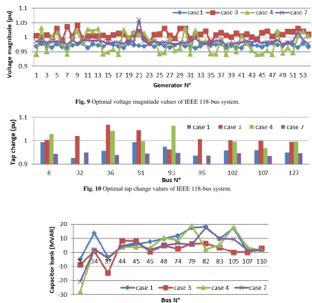
tap settings T and the capacitor banks obtained in the four cases are given in Figs. 9, 10 and 11. From this figures, we can see that all these results are between their minimum and maximum values.

5.4 DZ 114-Bus Power System

To demonstrate the applicability of the proposed MOALO algorithm in practical system; it has been examined and tested on the Algerian transmission network DZ 114-bus system [46]. This network is composed of 114 buses, 174 transmission lines, 15 generators, 16 transformers and 7 capacitor banks. It is

worth mentioning that bus number 04 is the slack bus and the total load demand is 3727 MW. The minimum and maximum limits of the voltage generator buses and load buses in this system are 0.9 pu and 1.1 pu [30]. For Algerian transmission network, there are 53 control variables (15 generator power outputs, 15 generator voltages, 16 transformers and 7 capacitor banks), these variables are to be optimized. The optimal outputs of power generation are represented in Table 10, the total fuel cost, power losses and the voltage deviation are also represented in this table. The rest of the optimal values are shown in Figs. 12, 13 and 14.

Fig. 9 Optimal voltage magnitude values of IEEE 118-bus system.

Fig. 10 Optimal tap change values of IEEE 118-bus system.

Fig. 11 Optimal capacitor bank values of IEEE 118-bus system.

(15)

Iranian Journal of Electrical and Electronic Engineering, Vol. 15, No. 1, March 2019 108 Table 10 Optimal results for the Algerian network DZ 114-bus power system.

Cases Min Case 01 Case 03 Case 04 Case 7 Max

Pg4 135.0000 458.0600 438.1300 427.64 420.9800 1350.0000

Pg5 135.0000 451,1905 531.4987 484.6373 485.1794 1350.0000

Pg11 10.0000 74,91904 86.3077 133.4379 173.8651 100.0000

Pg15 30.0000 212,0149 176.6917 122.1698 150.4472 300.0000

Pg17 135.0000 436,8922 430.6920 585.0619 575.4973 1350.0000

Pg19 34.5000 236,6123 193.8471 255.4143 170.3209 345.0000

Pg22 34.5000 197,7529 222.4540 229.9108 274.1317 345.0000

Pg52 34.5000 246,6429 310.5442 150.3864 145.2838 345.0000

Pg80 34.5000 171,7571 295.8228 279.1576 283.6721 345.0000

Pg83 30.0000 163,4842 207.0043 206.3403 123.0331 300.0000

Pg98 30.0000 214,0323 160.5078 223.5949 215.6620 300.0000

Pg100 60.0000 599,9999 454.8742 489.0052 504.7741 600.0000

Pg101 20.0000 199,9999 147.2013 101.6451 147.8956 200.0000

Pg109 10.0000 67,19996 61.0977 55.0481 77.9005 100.0000

Pg111 10.0000 81,96231 97.2401 73.6175 64.3927 100.0000

Fuel Cost [$/h] - 19355.8595 20600.7073 20910.3473 20360.0830 -

Ploss [MW] - - 66.0278 - 70.216 -

DV [pu] - - - 0.34066 0.6780 -

Fig. 12 The optimal voltage magnitude values of the Algerian network.

Fig. 13 The optimal tap change values of the Algerian network.

Fig. 14 The optimal capacitor bank values of the Algerian network.

(16)

We can see that all security constraints are checked for optimal voltage magnitudes, tap change values and capacitor bank (Figs. 12, 13 and 14).

Fig. 15 indicates that the proposed MOALO for DZ 114-bus system was successfully implemented the goal was to find the best different Pareto optimal front.

5.5 IEEE 300-Bus Test System

Finally, we have applied the MOALO to solve multiobjective optimal reactive power dispatch (MOORPD) problem considering large -scale power system IEEE 300 bus [44]. The MOORPD is an important issue in power system planning and operation. It is a well-known complex optimization problem with nonlinear characteristic. ORPD is formulated as multiobjective optimization problem, in which focuses to not only reduce transmission power losses, but also simultaneously minimizes the voltage stability index (L -index) or voltage deviation.

The objective of the voltage stability indices is to quantify how close a particular point is to the steady state voltage stability margin. These indices can be used on-line or offline to help operators in real time operation of power system.

The IEEE 300-bus test system, comprises 69 generators, 411 transmission lines including 107 transformers between and 14 compensators at the loads buses n° 96, 99, 133, 143, 145, 152, 158,169, 210, 217, 219, 227, 268 and 283.The total load active power of this system is (235.258 + j77.8797) pu at 100 MVA base.

The vector of control variables of IEEE 300-bus test system includes the magnitude voltages of generators, transformer tap settings and the capacitor banks. Table 11 represents the best result of a part of the vector of control which represents 14 compensators obtained from the MOALO algorithm for different cases. The Pareto-optimal solutions are illustrated in Fig. 16.

Based on the simulation results of different case studies, it is observed that the results demonstrate the potential of the proposed approach and show clearly its effectiveness to solve practical OPF. All results obtained do not violate the generation capacity constraints. It is important to note that the security constraints are satisfied for voltage magnitudes and line flows. No load bus is under its lower limit of 0.90 pu.

0 100 200 300 400 500

1.9 2 2.1 2.2 2.3

2.4x 10

4

Fuel cost ($/h)

It

e

ra

ti

o

n

2.059 2.06 2.061 2.062 2.063 2.064 2.065 x 104 65

65.5 66 66.5

Fuel cost ($/h)

P

o

w

e

r

lo

s

e

s

(

M

W

)

(a) (b)

0 1 2 3 4 5

x 104 0

0.5 1 1.5

Fuel cost ($/h)

V

o

lt

a

g

e

m

a

g

n

it

u

d

e

d

e

v

ia

ti

o

n

(

p

u

)

0

0.5

1 2

2.05 2.1 2.1560

70 80 90

Voltage magnitude deviation (pu) Fuel codt ($/h)

P

o

w

e

r

lo

s

e

s

(

M

W

)

(c) (d)

Fig. 15 Simulation results of the Algerian transmission network DZ 114-bus for (a) case 1 (b) case 3 (c) case 4 (d) case 7 using MOALO algorithm.

(17)

Iranian Journal of Electrical and Electronic Engineering, Vol. 15, No. 1, March 2019 110 Table 11 Optimal results of IEEE 300-bus power system for different cases.

Min Case: Ploss

Case: L_index

Case: DV

Case:

Ploss+L_index

Case:

Ploss+L_index+DV Max

Q96 0 411.8360 274.9774 96.4914 270.0682 343.9224 450

Q99 0 25.7816 27.7997 0.6444 41.7304 35.5968 59

Q133 0 47.3180 16.4863 0.9891 56.3709 27.5005 59

Q143 -450 -256.5247 -443.6522 -130.5488 -306.6606 -240.3758 0

Q145 -450 -414.5873 -97.8828 -447.0338 -374.6129 -184.4596 0

Q152 0 14.5335 45.0018 8.0079 58.0625 39.1839 59

Q158 0 41.8650 55.1477 5.7232 51.4768 40.3758 59

Q169 -250 -237.0456 -185.2194 -148.7700 -213.1328 -64.7152 0

Q210 -450 -436.9324 -445.5752 -376.7078 -279.7349 -169.4061 0

Q217 -450 -239.2131 -296.7490 -225.4550 -350.5397 -300.5593 0

Q219 -150 -141.3918 -100.4646 -58.4613 -110.3498 -51.1462 0

Q227 0 35.7928 44.9637 9.4773 43.7490 52.5504 59

Q268 0 12.9098 3.2247 12.1349 14.3013 7.6123 15

Q283 0 5.0810 9.4478 0.2379 12.1741 9.1863 15

Ploss(MW) - 363,4262 - - 384,3528 427,3942 -

L_index(pu) - - 0,14711 - 0,1564 0,1874 -

DV(pu) - - -- 1,3623 - 2,3780 -

410 420 430 440 450 460 470

0.18 0.19 0.2 0.21 0.22 0.23

Ploss (MW)

L

_

in

d

e

x

(

p

u

)

400

420 440

460 480

0.18 0.2 0.22 0.24

1 2 3 4

Ploss (MW) L__index (pu)

D

V

(p

u

)

(a) (b)

Fig. 16 Pareto-optimal solutions obtained for IEEE 300-bus power system; a) Case: Ploss+L_index and b) Case: Ploss+L_index+DV.

6 Conclusion

In this paper, a multiobjective optimal power flow problem (MOOPF) with four conflicting objectives; fuel cost, total emission, real power losses and magnitude voltage deviation under different constraints was solved using a recently developed MOALO algorithm. The proposed MOALO was applied to several cases studies in four power systems; namely IEEE 30-bus, IEEE 57-bus, IEEE 118-57-bus, IEEE 300-bus test systems and the Algerian network DZ 114-bus. The simulation results indicated that the proposed approach successfully achieved the goal of finding the best global settings of the control variables. The results obtained were compared with those obtained from two other algorithms namely MOMICA and MODA. The outcomes of the comparison confirm the effectiveness and the superiority of the proposed MOALO method in solving the optimal power flow (OPF) for small, medium and large scale electrical networks. Furthermore, MOALO has the ability more than the other algorithms (MOMICA, MODA) in solving the problems with more than two objective functions. Moreover, simulation results obviously demonstrate the capabilities of the proposed algorithm to generate a set of non-dominated feasible solutions.

Acknowledgement

This work was supported by Algerian Ministry of Higher Education and Scientific Research as part of the

projects PRFU under grant number

A01L07UN190120180008.

References

[1] H. Wang, C. E. Murillo-Sanchez, R. D. Zimmerman and R. J. Thomas , “On computational issues of market-based optimal power flow,” IEEE Transactions on Power Systems, Vol. 22, No. 3, pp. 1185–1193, 2007.

[2] R. Datta, K. Deb, and A. Segev, “A bi-objective hybrid constrained optimization (HyCon) method using a multi-objective and penalty function approach,” in IEEE Congress on Evolutionary Computation (CEC),pp. 317–324,2017.

[3] W. D. Rosehart, C. A. Canizares, and V. H. Quintana, “Multiobjective optimal power flows to evaluate voltage security costs in power networks,” IEEE Transactions on Power Systems, Vol. 18, No. 2, pp. 578–587, May 2003.

(18)

[4] V. C. Ramesh and X. Li, “A fuzzy multiobjective approach to contingency constrained OPF,” IEEE Transactions on Power Systems, Vol. 12, No. 3, pp. 1348–1354, 1997.

[5] M. A. Abido, “A novel multiobjective evolutionary algorithm for environmental/economic power dispatch,” Electric Power Systems Research, Vol. 65, No. 1, pp. 71–81, 2003.

[6] A. F. Attia, Y. A. Turki, and A. M. Abusorrah, “Optimal power flow using adapted genetic algorithm with adjusting population size,” Electric Power Components and Systems, Vol. 40, No. 11, pp. 1285–1299, 2012.

[7] S. Balasubramanian, R. V. Gokhale, and A. Sekar, “A new AC optimal power flow formulation and solution using Genetic Algorithm based on P-Q decomposition,” in North American Power Symposium (NAPS), pp. 1–5, Oct. 2015.

[8] S. Almasabi, F. T. Alharbi, and J. Mitra, “Opposition-based elitist real genetic algorithm for optimal power flow,” in North American Power Symposium (NAPS), pp. 1–6, Sep. 2016.

[9] Y. Zeng and Y. Sun, “Solving multiobjective optimal reactive power dispatch using improved multiobjective particle swarm optimization”, in The 26th_{Chinese, Control and Decision Conference,}

pp. 1010–1015, May 2014.

[10] K. Price, R. Storn, and J. Lampinen, Differential evolution: A practical approach to global optimization. Berlin, Germany: Springer-Verlag, 2005.

[11]D. Karaboga, “An idea based on honey bee swarm for numerical optimization,” Technical Report-TR06, Erciyes University of Engineering, Faculty of Computer Engineering Department, Oct. 2005.

[12] D. Simon, “Biogeography-based optimization,” IEEE Transactions on Evolutionary Computation, Vol. 12, No. 6, pp. 702–713, Dec. 2008.

[13]A. Bhattacharya and P. k. Chattopadhya, “Biogeaography-based optimization for different economic load dispatch problems,” IEEE Transactions on Power Systems, Vol. 25, No. 2, pp. 1064–1077, May 2010.

[14]H. Nobahari, M. Nikusokhan, and P. Siarry, “Nondominated sorting gravitational search algorithm,” in Proc. of the 2011 International Conference on Swarm Intelligence (ICSI), pp. 1–10, 2011.

[15]A. Hatamlou, “Black hole: A new heuristic optimization approach for data clustering,” Information Sciences, Vol. 222, pp. 175–184, 2013.

[16]Omid Bozorg-Haddad, Advanced optimization by nature-inspired algorithms. Springer Singapore, 2018.

[17]S. Mirjalili, “Dragonfly algorithm: a new metaheuristic optimization technique for solving single objective, discrete, and multi-objective problems,” Neural Computing and Applications, Vol. 27, No. 4, pp. 1053–1073, 2016.

[18]M. Ghasemi, S. Ghavidel, M. M. Ghanbarian, M. Gharibzadeh, and A. A. Vahed, “Multi-objective optimal power flow considering the cost, emission, voltage deviation and power losses using multi-objective modified imperialist competitive algorithm,” Energy, Vol. 78, pp. 276–289, 2014.

[19]M. Ding, H. Chen, N. Lin, S. Jing, F. Liang, X. Fang, and W. Liu, “Dynamic population artificial bee colony algorithm for multi-objective optimal power flow,” Saudi Journal of Biological Sciences, Vol. 24, No. 3, pp. 703–710, Mar. 2017.

[20]W. Warid, H. Hizam, N. Mariun, and N. I. A. Wahab, “A novel quasi-oppositional modified Jaya algorithm for multi-objective optimal power flow solution,” Applied Soft Computing Journal, Vol. 65, pp. 360–373, Apr. 2018

[21]O. Herbadji, L. Slimani, and T. Bouktir, “Multi-objective optimal power flow considering the fuel cost, emission, voltage deviation and power losses using multi-objective dragonfly algorithm”, in International Conference on Recent Advances in Electrical Systems, pp. 191–197, 2017.

[22]S. Mirjalili, P. Jangir, and S. Saremi, “Multi-objective ant lion optimizer: a multi-“Multi-objective optimization algorithm for solving engineering problems,” Applied Intelligence, Vol. 46, No. 1, pp. 79–95, 2017.

[23]E. Atashpaz-Gargari and C. Lucas, “Imperialist competitive algorithm: An algorithm for

optimization inspired by imperialistic

competition”, in IEEE Congress on Evolutionary Computation, pp. 4661–4666, 2007.

[24]J. Hazra and A. K. Sinha, “A multi-objective optimal power flow using particle swarm optimization”, European Transaction on Electrical Power, Vol. 21, No. 1, pp. 1028–1045, 2011. [25] A. J. Wood and B. F. Wollenberg, Power

Generation Operation and Control-2nd Edition. in Fuel and Energy Abstract, Vol. 3, No. 37, 1996. [26]G. W. Stagg and A. H. El-Abiad, Computer

methods in power systems analysis. New York: McGraw-Hill, 1968.

(19)

[27]L. Slimani and T. Bouktir, “Economic power dispatch of power system with pollution control using multiobjective ant colony optimization,” International Journal of Computational Intelligence Research, Vol. 3, No. 2, pp. 145–153, 2007.

[28] M. S. Kumari and S. Maheswarap, “Enhanced genetic algorithm based computation technique for multi-objective optimal power flow solution,” International Journal of Electrical Power and Energy Systems, Vol. 32, No. 6, pp.736–742, 2010. [29]L. Slimani and T. Bouktir, “Optimal power flow

solution of the Algerian electrical network using differential evolution algorithm,” Telkomnika Journal, Vol. 10, No. 2, pp. 199–210, 2012.

[30]K. Y. Lee, Y. M. Park, and J. L. Ortiz, “A united approach to optimal real and reactive power dispatch”, IEEE Transactions on Power Apparatus and System, No. 5, pp. 42–43, 1985.

[31]Y. Xu, S. Member, W. Zhang, S. W. Liu and F. Ferrese, “Multiagent-based reinforcement learning for optimal reactive power dispatch”,IEEE Transactions on Systems, Vol.42, No. 6, pp. 1742– 1751, 2012.

[32] J. T. Ma and L. L. Lai, “Application of genetic algorithm to optimal reactive power dispatching

voltage-dependent load models,” in IEEE

International Conference on Evolutionary Computation, Vol. 1, pp. 5–10, 1995.

[33]H. R. E. H. Bouchekara, M. A. Abido, and A. E. Chaib, “Optimal power flow using an improved electromagnetism-like mechanism method”, Electric Power Components Systems, Vol. 44, No. 4, pp. 434–449, 2016.

[34]H. R. E. H. Bouchekara, M. A. Abido, A. E. Chaib, and R. Mehasni, “Optimal power flow using the league championship algorithm: A case study of the Algerian power system,” Energy Conversion Management, Vol. 87, pp. 58–70, 2014.

[35]B. Bentouati, S. Chettih, and L. Chaib, “Interior search algorithm for optimal power ﬂow with non-smooth cost functions,” Cogent Engineering, Vol. 4, No. 1, 2017.

[36]A. A. A. El Ela, M. A. Abido, and S. R. Spea, “Optimal power flow using differential evolution algorithm,” Electric Power Systems Research, Vol. 80, No. 7, pp. 878–885, 2010.

[37]H. R. E. H. Bouchekara, “Optimal power flow using black-hole-based optimization approach,” Applied Soft Computing, Vol. 24, pp. 879–888, 2014.

[38]K. Vaisakh and L. R. Srinivas, “A genetic evolving ant direction DE for OPF with non-smooth cost functions and statistical analysis,” Energy, Vol. 35, No. 8, pp. 3155–3171, 2010.

[39]K. Vaisakh and L. R. Srinivas, “Evolving ant direction differential evolution for OPF with non-smooth cost functions,”, Engineering Application of Artificial Intelligence, Vol. 24, No. 3, pp. 426–436, 2011.

[40] M. A. Abido, “Optimal power flow using particle swarm optimization”, International Journal of Electrical Power Energy Systems, Vol. 24, No. 7, pp. 563–571, 2002.

[41]R. H. Liang, S. R Tsai, Y. T. Chen, and W. T. Seng, “Optimal power flow by a fuzzy based hybrid particle swarm optimization approach,” Electric Power Systems, Vol. 81, No. 7, pp.1466–1474, 2011.

[42]L. L. Lai, J. T. Ma, R. Yokoyama, and M. Zhao, “Improved genetic algorithms for optimal power flow under both normal and contingent operation states,” International Journal of Electrical Power and Energy Systems, Vol. 19, No. 5, pp. 287–292, 1997.

[43]M. A. Medina, S. Das, C. A. C. Coello, and J. M. Ramírez, “Decomposition-based modern metaheuristic algorithms for multi-objective optimal power flow – A comparative study,” Engineering Applications of Artificial Intell