Eric Canc`es & Jean-Fr´ed´eric Gerbeau, Editors DOI: 10.1051/proc:2005014
PARAMETER IDENTIFICATION FOR A ONE-DIMENSIONAL BLOOD FLOW
MODEL
∗Vincent Martin
1, Francois Cl´
ement
2, Astrid Decoene
3and Jean-Fr´
ed´
eric
Gerbeau
4Abstract. The purpose of this work is to use a variational method to identify some of the parameters of one-dimensional models for blood flow in arteries. These parameters can be fit to approach as much as possible some data coming from experimental measurements or from numerical simulations performed using more complex models.
A nonlinear least squares approach to parameter estimation was taken, based on the optimization of a cost function. The resolution of such an optimization problem generally requires the efficient and accurate computation of the gradient of the cost function with respect to the parameters.
This gradient is computed analytically when the one-dimensional hyperbolic model is discretized with a second order Taylor-Galerkin scheme. An adjoint approach was used.
Some preliminary numerical tests are shown. In these simulations, we mainly focused on deter-mining a parameter that is linked to the mechanical properties of the arterial walls, the compliance. The synthetic data we used to estimate the parameter were obtained from a numerical computation performed with a more accurate model: a three-dimensional fluid-structure interaction model. The first results seem to be promising. In particular, it is worth noticing that the estimated compliance which gives the best fit is quite different from the values that are commonly used in practice.
R´esum´e. Le but de ce travail est d’identifier certains des param`etres existant dans des mod`eles 1-d d’´ecoulement sanguin dans des art`eres. Ces param`etres peuvent permettre d’approcher autant que possible des configurations g´eom´etriques r´ealistes ou des donn´ees exp´erimentales. Une approche de l’estimation de param`etres par moindres carr´es non-lin´eaires a ´et´e adopt´ee, bas´ee sur l’optimisation d’une certaine fonction coˆut. La r´esolution d’un tel probl`eme de minimisation requiert le calcul efficace et pr´ecis du gradient de la fonction coˆut par rapport aux param`etres. Le gradient est discr´etis´e analytiquement dans le cas d’une discr´etisation du mod`ele hyperbolique 1-d par le schema de Taylor-Galerkin. Une approche par l’´etat adjoint a ´et´e employ´ee.
Des premiers r´esultats num´eriques sont fournis. Pour ces simulations, nous nous sommes concentr´es sur la d´etermination d’un param`etre li´e aux propri´et´es m´ecaniques de la paroi art´erielle. Les donn´ees synth´etiques utilis´ees pour l’estimation de ce param`etre ont ´et´e obtenues `a partir d’un mod`ele beaucoup plus raffin´e : un mod`ele 3-d d’interaction fluide-structure. Les r´esultats semblent int´eressants car le param`etre estim´e est assez diff´erent de ce `a quoi on s’attendraita priori.
∗This study was supported by RTN-Project “HaeMOdel”, project no HPRN-CT-2002-00270.
1MOX, Dpto di Matematica, Politecnico di Milano, Via Bonardi 9, 20133 Milano, Italy ;
e-mail: [email protected] & [email protected]
2Estime, Inria Rocquencourt, BP 105, 78153 Le Chesnay, France ; e-mail:[email protected] 3Bang, Inria Rocquencourt, BP 105, 78153 Le Chesnay, France ; e-mail: [email protected] 4Reo, Inria Rocquencourt, BP 105, 78153 Le Chesnay, France ; e-mail:[email protected]
c
EDP Sciences, SMAI 2005
Introduction
We focus in this study on the parameter estimation of a 1-d blood flow model, [11, 19]:
∂A ∂t +
∂Q
∂z = 0, ∂Q
∂t + ∂ ∂z
αQ2 A
+A
ρ ∂P
∂z +Kr
Q A
= 0,
where the pressureP, the area A and the flux Q are the unknowns of the problem. We denoted by z the abscissa, t the time, ρ the density of the blood. Two parameters, the Coriolis coefficient α and the friction parameterKr, are introduced in this model. This system is closed with a wall displacement law of the form
P(t, z)−Pext= ˜β
A1/2−A10/2
,
that links the pressure and the area. We introduced the external pressure Pext, the area at rest A0 and a coefficient ˜β that takes into account the mechanical characteristics of the arterial wall. The parameters (α,β, K˜ r, A0) used in this model are related to physiological data or to the velocity profile. Thus our aim is to identify some of these parameters.
Motivations. Two main objectives can be thought of to motivate the parameter estimation in 1-d models. The first goal may have interesting clinical applications. Knowing some non-invasive clinical data measured on a patient, one would like to retrieve the actual physiological or mechanical constants of this patient. For instance, it is possible to measure unintrusively the mean fluxes and areas as a function of time at two or three different sections of an artery. From these data, one would like to identify the mechanical properties of the arterial wall: we could thus obtain the compliance of the wall and the pressure in a totally non-invasive manner.
The second objective is consists in making a coarsening of models. One is now able to solve the full 3-d fluid structure interaction problem on real geometries, coming from real patients. However the resolution of this problem is quite expensive and this complex model cannot probably be afforded for an intensive numerical study requiring lots of resolutions. This can occur when one wishes to modify the configuration of the flux or the boundary conditions for instance. In this case, a single resolution of the accurate but expensive 3-d model could provide data, such as the flux and the area for all sections of the mesh. Then one can estimate the 1-d parametersfrom the 3-d data; this would allow to make use of the cheap 1-d model for intensive computations, but using the parameters that take into account data coming from a real geometry and a physically more detailed model. This multiscale approach has already been used in a medical application: some 3-d Navier-Stokes (without compliant walls) were performed to obtain a simple numerical/experimental law that was used in ulterior 0-d simulations, [16, 17]. The difference is that in this study, we base our parameter identification on sound mathematical tools, and we focus on 1-d models that provide a more accurate description of wave propagation in the large arteries. One of the conclusions of this work is that the coefficient estimated by solving the inverse problem is quite different from the coefficient one would have chosena priori(ana prioriexpression for ˜β is provided in Section 1). Thus this approach could provide 1-d models that are suitable for a 3-d–1-d coupling in multiscale computations, see [8]. This illustrates the relevance of our approach.
To conclude on the motivations, one can either aim at estimating physical parameters from experimental unintrusive measurements, or at having a cheap 1-d model to be as close as possible to an expensive 3-d model, in order to make realistic configuration studies using this cheap model. We note here that the methodology remains identical for both objectives, the only difference being the expression of the measurement operator.
is, as expected, a linear 1-d hyperbolic system, but has nonstandard discretization and boundary conditions, that are due to the differentiation of the Taylor-Galerkin scheme.
A previous attempt was made in [14] to estimate the elasticity of the arteries. However, instead of differen-tiating the discrete equations as we do here, the author differentiated first the continuous equations and then discretized the continuous adjoint problem thus obtained. We believe this is a possible reason for the very slow convergence he reached in the minimization process (about 1500 iterations for three parameters).
Finally, this approach allows to make a sensitivity analysis, [13, 15], that can provide information on the relevant parameters to estimate, and on the type of measurements to perform. But this goes beyond the scope of this study.
Results. The analytical discrete gradient was implemented and validated by comparison with finite differences approximations. The adjoint problem was not computed by automatic code differentiation, but directly im-plemented. Thus we could easily control the memory required by the gradient code. We used a constrained optimization code based on a quasi-Newton method with active constraints.
We present some preliminary numerical results. In these numerical simulations, we mainly focused on deter-mining the parameter ˜β that is linked to the mechanical properties, i.e. the compliance, of the arterial walls. The synthetic data we used to estimate the parameter were obtained from a numerical computation performed with a 3-d fluid structure interaction model. We first used as data the values of the areas and fluxes at only two or three points of the domain (boundaries plus maybe the middle point). Although the data at two points do not seem to be enough to find a stable value, it seems that with three points, one can obtain a ˜β relatively stable (i.e. it is little changed when the estimation is made with all available spatial data). In the second numerical tests, we used all data available from the 3-d computation. These first numerical results seem promising and should be followed by further developments.
In Section 1, we present briefly the continuous 1-d model, that is derived in Section 2 with the Taylor-Galerkin scheme. In Section 3, the gradient of the least squares cost function is computed with the adjoint approach. Numerical results are presented in Section 4, and some conclusions and perspectives in Section 5.
1.
Direct model: 1-d blood flow model
We present in this section a 1-d blood flow model based on the works in [10, 20]. See also [19]. It is a 1-d vectorial hyperbolic problem, with a 2×2 flux matrix that admits two real eigenvalues with opposite signs under physiological conditions.
We leave the problem of the parameterization and of the measurements for the next sections, see Section 3.1.
1.1.
Continuous blood flow model
Let Ω = (0, L) be a 1-d domain of lengthL >0. LetI= (0, Tf), withTf >0, the time interval of simulation. The continuous system of equations reads, for the abscissaz∈Ω and the timet∈I
∂A ∂t +
∂Q
∂z = 0, z∈Ω, t∈I, ∂Q
∂t + ∂ ∂z
αQ2 A
+A
ρ ∂P
∂z +Kr
Q A
= 0, z∈Ω, t∈I,
(1)
whereU= [A, Q]is the vectorial unknown of the problem, made of the areaAand of the fluxQ. The pressure
P is an intermediary unknown. We denoted by ρthe blood density that we assume perfeclty known in this study. Two parameters, the Coriolis coefficientαand the friction parameterKr, are introduced when deriving this model. This system of partial differential equations is completed with an initial condition
and some adapted boundary conditions
φ0(U(t,0),p) = q0(t), t∈I,
φL(U(t, L),p) = qL(t), t∈I . (3)
In equations (2) and (3),U0,q0 andqL are given initial and boundary data. The definition of the real-valued boundary functionsφ0, φL is discussed in Section 2.2.
The system (1) is closed with a wall displacement law of the form, see [21] for instance and the reference therein,
P(t, z)−Pext=ψ(A;A0,β) =β0
A A0
β1 −1
, (4)
whereβ = (β0, β1) is a pair of positive real parameters. The power coefficient β1 is often taken equal to 1/2, which means that the pressure difference is proportional to the wall displacement, and, in this case, a linear elastic law can provide an expression forβ0, if the mechanical properties of the arterial wall are knowna priori,
β1= 1/2, β0=
√ πh0,wE
√
A0(1−ν2), (5)
where h0,w is the wall thickness, E is the wall Young modulus, and ν is the Poisson coefficient. We can reformulate the wall displacement law in the following way:
P(t, z)−Pext=ψ(A;A0, β) = 2ρβ
A1/2−A10/2
, with β= β0 2ρA0 =
√ πh0,wE
2ρA0(1−ν2). (6)
We introduce the following quantity
c=c(A;A0,β) = A
ρ ∂ψ ∂A =
β0β1 ρ
A A0
β1
, (7)
which has the dimension of a velocity and is related to the speed of propagation of simple waves along the tube. We also introduce the integral of the square of the celeritycwith respect to the area
C(A;A0,β) =
A
A0
c2(τ;A0,β)dτ = β0β1A0
ρ(β1+ 1)
A A0
β1+1 −1
. (8)
Defining the flux function
F(U,p) =
Q
αQ
2
A +C
(9)
and the source term
B(U,p) =
0
B2
, B2=Kr
Q A+
A ρ
∂ψ ∂A0
dA0
dz + A
ρ ∂ψ ∂β
dβ dz −
∂C ∂A0
dA0
dz − ∂C ∂β
dβ
dz , (10)
we can write the complete problem in a conservative form
∂U
∂t + ∂
We introduce the jacobian matrix
H(U,p) = ∂F
∂U =
0 1
c2−α
Q A
2
2αQ A
, (12)
whose eigenvalues are real, distinct, see [19]. It is also noted that for common values of the blood flow in human arteries, these eigenvalues haveopposite signs. We assume in the rest of the article that this hypothesis holds.
Remark 1.1. We can make two remarks concerning the initial and boundary terms. First, when simulating a phenomenon that is periodic in time such as the arterial flow, the initial dataU0 should not interfere on the results. Therefore we did not consider it as one of the parameters to be estimated.
Second, as already noticed, the boundary conditions must be properly chosen. The number of boundary conditions to impose at each end of the vessel equals the number of characteristics entering the domain through that boundary. As the eigenvalues are distinct with opposite signs, i.e. the flow is sub-critical everywhere, one must impose exactlyone scalar boundary condition at z= 0 andz=L, see [19].
Thus the boundary conditions in equation (3) are correctly set, provided that the scalar functionsφ0, φLare properly chosen.
2.
Discrete blood flow model
In this section, we give the discretization of the continuous problem (11).
In the rest of this article, the upper-scripts will be devoted to time steps numbers, whereas the lower indices will in general denote the space indices, or the component index of a vector. For instance, for a vectorv, the
αth component ofv at timetn and at abscissaz
iwill be denoted (vα)ni.
2.1.
Taylor-Galerkin scheme
We discretize our system by a second order Taylor-Galerkin scheme [1], which might be seen as the finite element counterpart of the Lax-Wendroff scheme. It has been chosen for its excellent dispersion error character-istic and its relative simplicity of implementation. See [11] for details concerning the derivation of the scheme for the blood flow model.
Let the interval Ω = (0, L) be subdivided into N + 1 elements ei+1
2 = [zi, zi+1], for i = 0, . . . , N and
zi+1 =zi+hi+12, with z0 = 0, and
N
i=0hi+12 =L, where hi+12 >0 is the local element size. Let h >0 be the smallest diameter of all elementsei+1
2, i= 0, . . . , N. We discretize the time intervalI= (0, Tf) in the same
way: let (tn), n= 0, . . . , Nt, beNt+ 1 instants such that t0= 0< . . . < tn < tn+1 < . . . < tNt =Tf. We call ∆tn+12 =tn+1−tn>0 the time step betweentn andtn+1, n= 0, . . . , Nt−1.
The space discretization is carried out using the finite element method [18]. Let Ψhbe the space of continuous piecewise linear finite element functions, also denoted P1, and Ψh = [Ψh]2, while Ψh,0 = [Ψh,0]2 = {ψh ∈
Ψh|ψh = 0atz = 0 andz = L}. Let ψi be the P1 linear finite element nodal function associated to the node at z = zi, i = i = 0, . . . , N + 1. Thus one can write Ψh = span{ψi, i= 0, . . . , N+ 1} while Ψh,0 = span{ψi, i= 1, . . . , N}. We will denote a generic vector valued test function by ψh ∈ Ψh. The discrete continuity and momentum equations are recovered by taking test functions of the form ψh = [ψh,0]T and
ψh= [0, ψh]T, respectively, withψh∈Ψh,0.
At each time step we seek the solution Uh ∈ Ψh that we may write Unh(z, t) = Ni=0+1Uniψi(z, t), with Uni = [Ani, Qin] the approximation ofAandQat mesh nodezi.
Introducing the notations forU∈Ψh, BU= ∂B
∂U,
FnLW(U) =F(U)−∆t n+12
2 H(U)B(U) and B n
LW(U) =B(U)− ∆tn+12
2 BU(U)B(U), we write in equation (13) the Taylor-Galerkin discretization of the problem (11).
Given U0h, forn= 0,1, . . . , Nt−1, findUnh+1∈Ψhsuch that for allψh∈Ψh,0
(Unh+1,ψh)Ω = (Unh,ψh)Ω+ ∆tn+12
FnLW(Unh),dψh dz
Ω−
(BnLW(Unh),ψh)Ω
+(∆t n+1
2)2
2
−
H(Unh)∂F
∂z(U
n h),
dψh dz
Ω
+
BU(Unh)∂F(U n h)
∂z ,ψh
Ω
,
+B.C.z= 0 equation onUnh+1(0),
+B.C.z=L equation onUnh+1(L).
(13)
In the system (13), by taking internal test functionsψh = [ψi,0]T and ψh = [0, ψi]T, for i = 1, . . . N, we obtain N discrete equations for continuity and momentum, respectively, for a total of 2(N + 2) unknowns (Ai andQifori= 0, . . . , N+ 1). Thus boundary and compatibility conditions have to provide four additional scalar relations, see next section.
To fully discretize the equation in (13), we need to determine how the non-linear terms are computed and which numerical integration is performed. We choose to approximate the vectors F and B depending on
Unh in (13) in the space P1, and the matrices H and BU in the space of element-wise constant functions
P0,h :=
vh∈L2(Ω)|vh|ei+ 1
2 = cst, i= 0, . . . , N
. With this hypothesis, the integrations in (13) can easily be made exactly.
Thus for a vectorial functionv:Ψh→R2,U→v(U) = [v1, v2], we define
vh(U) =
N+1
i=0
v1(Ui)ψi , N+1
i=0
v2(Ui)ψi
∈Ψh,
and for a matrixM :Ψh→R2×2,U→M(U) = (Mαβ)α,β=1,2, we define
Mh(U) = (Mh,αβ(U))α,β=1,2, Mh,αβ(U) = N
i=0 ˜
Mh,αβ, i+1
21i+12 ∈P0,h (14)
with the mean value ˜Mh,αβ, i+1 2 =
1
2(Mαβ(Ui) +Mαβ(Ui+1)) over the element ei+1
2 = [zi, zi+1], and the
characteristic function 1i+1
2 of the interval [zi, zi+1], fori= 0, . . . , N.
With these notations, we can write the fully discretized Taylor-Galerkin scheme (13). Using the notation
Fnh,LW(U) =Fh(U)−∆t n+1
2
2 Hh(U)Bh(U) and Bh,LW(U) =Bh(U)− ∆tn+1
2
2 (BU)h(U)Bh(U), and introducing the operator forU,W∈Ψh
anh(U,W;p) = ∆tn+12
Fnh,LW(U),dW dz
Ω−
Bnh,LW(U),W
Ω
+(∆t n+12)2
2
−
Hh(U)∂Fh
∂z (U), dW dz Ω +
(BU)h(U)∂Fh
∂z (U),W
Ω
,
the fully discretized scheme (13) yields: GivenU0h∈Ψh, findUh:= (Un
h)n=1,...,Nt ∈(Ψh)Nt such that forn= 0,1, . . . , Nt−1 (Unh+1,ψh)Ω = (Un
h,ψh)Ω+anh(Unh,ψh;p) ∀ψh∈Ψh,0 ,
B.C. onUnh,+10 ,
B.C. onUnh,N+1+1.
(16)
In the discrete approximate problem (16), all the integrals can be computed exactly as they involve only the products of two functions belonging either toP1 or toP0.
We need to add boundary conditions and compatibility conditions atz= 0 andz=Lto close the system.
2.2.
Boundary conditions
In this section and in the next sections 2.3 and 2.4, we will omit the subscripthin the variable names, for the sake of simplicity.
As noticed in Remark 1.1, the hyperbolic problem (11) is well posed under sub-critical flow hypothesis when one imposes as boundary conditions one scalar equation at each side of the tube. These conditions can be the prescribed incoming characteristics, the prescribed pressure or the prescribed flux, for instance. It is not possible to impose exactly at the same boundary both the flux and the pressure, see [11].
We decide to give a flux at the inlet and a pressure at the outlet:
Qn0+1 = φ0(q0(tn+1),p) =q
0(tn+1)
AnN+1+1 = φL(pL(tn+1),p),
(17)
where q0 is the flux and pL is the pressure to be imposed at the boundaries, whereas φi, i = 0, L are given functions. The functionφ0 is in this case the identity, and φL transforms the given pressurepL at the outlet
into the conservative unknownA. With the pressure law (4), it becomesA=φL(pL,p) =A0
1 +pL
β0
1/β1
.
2.3.
Compatibility conditions
To close the discrete system we need two more conditions on the boundaries. These conditions are a numerical artefact that is linked to the type of scheme we adopted. They are called compatibility conditions and are chosen to be non-reflecting conditions at each side of the tube. We assume that these conditions are treated explicitly and linearly, imposing some conditions on the pseudo-characteristic variables, [19]. Thus they can take the following form:
l2(Un)Un0+1−T2(Un) = 0 atz= 0,
l1(Un)Un+1
N+1−T1(Un) = 0 atz=L,
(18)
whereli(Un)∈R2, i= 1,2 are the two left eigenvectors depending onUn associated to the matrixH defined in equation (12), andT1andT2 are some scalar functions depending onUn.
2.4.
Fully discretized problem
Gathering the boundary and compatibility conditions (17) and (18) and reintroducing the parametersp, we obtain
Θ0(Un,p)U0n+1−T0(Un,p) = 0 ΘL(Un,p)Un+1
N+1−TL(Un,p) = 0 ,
(19)
with atz=z0= 0
Θ0(Un,p) =
Θ0,1 Θ0,2(Un,p)
=
0 1
l2(Un,p)
, T0(Un,p) =
q0(tn+1)
T2(Un,p)
and atz=zN+1=L
ΘL(Un,p) =
ΘL,1(Un,p) ΘL,2
=
l1(Un,p) 1 0
, TL(Un,p) =
T1(Un,p)
φL(pL(tn+1),p)
.
Finally, reintroducing the subscripth, adding the boundary and compatibility conditions (19) to the com-pletely discretized scheme (16), the problem to be solved reads:
GivenU0h∈Ψh, findUh:= (Un
h)n=1,...,Nt ∈(Ψh)Nt such that forn= 0,1, . . . , Nt−1 (Unh+1,ψh)Ω = (Un
h,ψh)Ω+anh(Unh,ψh;p) ∀ψh∈Ψh,0,
Θ0(Unh,p)Uh,n+10 = T0(Unh,p),
ΘL(Un
h,p)Unh,N+1+1 = TL(Unh,p).
(20)
Remark 2.1. The problem (11) is a 1-d nonlinear hyperbolic problem, but the Taylor-Galerkin discretiza-tion (20) contains (second order) parabolic terms. Thus, one needs to impose not only the boundary condi-tions (17) that are natural for a hyperbolic problem, but also the compatibility condicondi-tions (18). Therefore at each time step, before computing the solution at internal nodes, one has to compute the boundary valuesUnh,+10
andUnh,N+1+1, by solving the two (2×2) linear systems (19).
3.
Gradient of the discrete problem
We present in this section the gradient of the discrete problem (20) using the adjoint approach. We recall that we used and implemented the rule (advocated in [3], [4], [5]): disretize first, differentiate after. In Section 3.1, some notations are defined in order to present briefly in Section 3.2 the adjoint state approach, and to compute analytically the gradient in Section 3.3.
3.1.
Forward operators
3.1.1. State equation
The equation (20) defines astateequation that relates the parameterspto the state variablesUh
E(p,Uh) = 0, (21)
where the parameters are
p= (α, β0, β1, Kr, A0, q0, qL) ∈RP , (22) with the dimensionP >0 of the parameter space to be defined further, and the state variable are
Uh= (Unh)n=1,...,Nt =
[Ani, Qni]i=0,...,N+1;n=1,...,N
t ∈(Ψh)
Nt =RN, N = 2N
t(N+ 2). (23)
In equation (23), we have assimilated the finite functional space (Ψh)Nt and the spaceRN. It will also be done
forΨh and R2(N+2). In the rest of the article, for simplicity but with an abuse of notation, we may use the same notation Wn
h for an element ofΨh or ofR2(N+2).
As there exists a unique solutionUp, hto the problem (21) for a given set of parametersp, see [11], we can define the direct application
ϕ:RP −→ RN,
p −→ ϕ(p) =Up, h, (24)
3.1.2. Measurement operator
LetM be a measurement (or observation) operator
M :RN −→ RM,
U −→ M(U) =V, (25)
withM>0 the dimension of the measurement space. Different measurement operators can be devised, linear or nonlinear, according to the type of data that are provided.
For instance, an experiment could provide the flux and area of a vessel at two different pointsζ0< ζ1, ζ1−ζ0=
L, at given (Vt+ 1) instants θ0 = 0< . . . < θν < θν+1 < . . . < θVt =T
f. It is then reasonable to perform the 1-d simulation between these two points, and therefore take z0 = ζ0 and zN+1 = ζ1. One can also assume for simplicity that the temporal discretization is chosen such that the instants (θν)
ν=0,...,Vt constitutes
a subsequence of (tn)
n=0,...,Nt. Therefore, letφt:{0,1, . . . ,Vt} → {0,1, . . . , Nt}be the increasing function such thattφt(ν)=θν, withφ
t(0) = 0 and φt(Vt) =Nt. With these hypotheses, the measurement operator is simply a weighted sampling of the direct solutionUp, h. It is linear and can be expressed
M(U) =
[wAi,ν Aφit(ν), wQi,νQφit(ν)]
i=0andN+1;ν=0,...,Vt
and M= 2×(Vt+ 1)×2,
where the coefficientswA
i,ν and wQi,ν are positive weights attributed to each measure, representing the “degree of confidence”, i.e. the inverse of the incertainty, one has in this measure.
When the data come from a numerical 3-d fluid structure computation, one can exploit the numerical results on (Vz+ 1) internal sections (ζj)j=0,...,Vz of the 3-d domain: Vz = 1,2 or more. In this case, apply the same technique for the spatial discretization as the one shown above for the temporal sampling, and introduce the increasing indexation functionφz in the same manner asφt. The measurement operator becomes this time
M(U) =
[wAj,ν Aφφt(ν) z(j), wj,νQ Q
φt(ν)
φz(j)]
j=0,...,Vz;ν=0,...,Vt
and M= 2(Vt+ 1)(Vz+ 1), (26)
with the positive weightswj,νA andwQj,ν, j= 0, . . . ,Vz; ν= 0, . . . ,Vt.
3.1.3. Forward function
LetF =M◦ϕbe the forward function, from the parameter space to the measure space
F :RP −→ RM,
p −→ F(p) =Vp, h=M(Up, h) =M(ϕ(p)). (27)
3.1.4. Cost function
The resolution of the inverse problem consists in minimizing a cost function that computes the least squares error between the measured data and the numerical results computed with the 1-d model. Thus the inverse problem amounts to an optimization problem. To solve it, it is necessary to define the cost function to minimize, that depends on the type of problem under consideration. Then one must choose an adequate technique to perform the minimization of this cost function.
We assume that the measurement operator is defined by (26). Consider a given data vectorZ∈RM and we callZw∈RM this vector multiplied by the positive weights introduced in (26),
Z= ([Adνj, Qdνj])j=0,...,Vz;ν=0,...,Vt ∈RM , Zw= ([wAj,ν Adνj, wj,νQ Qdνj])j=0,...,Vz;ν=0,...,Vt ∈RM ,
where Adν
LetJ be the cost function
J :RP −→ R,
p −→ J(p) = 1
2Zw−M(Up, h)
2
RM , (28)
where · Rn is the discretel2norm inRn, associated with the scalar product<·,·>Rn,n >0. The cost function can be expressed easily, withUp, h= ([An
i, Qni])∈RN,
J(p) =1 2
Vt
ν=0 Vz
j=0
(wj,νA )2
Adνj −Aφφt(ν) z(j)
2
+ (wQj,ν)2
Qdνj −Qφφt(ν) z(j)
2
. (29)
3.1.5. Parameterization
It is important to define the parameterization properly, see [6], and a sensitivity analysis can provide some information on this matter. In this section, we consider a general parameterization. The parameters are only supposed to satisfy some constraints determined by some physiological considerations, such that the parameters
pbelong to a subsetC ofRP.
3.2.
Optimization: adjoint state approach
In order to perform correctly the optimization of the cost function (28) with a descent method, one needs to compute the gradient of the cost function in a fast and accurate way. It is known that the finite difference method is not efficient, see [4, 13]. One could rely on adirect computation of the jacobian of the forward map
F, with a cost that is proportional to the numberP of parameters. We decided to compute the gradient using an adjoint state approach that we present briefly here. As in our numerical experiments, see section 4, the number of parameters to identify is very low, we could have fruitfully taken the former approach. However, we preferred the adjoint method, that allows to identify, in a second step, more parameters, with a cost that remains independent of the dimension of the parameter space.
To compute the gradient of a functionG=G(p,V) which is anexplicit function of the parameter vectorp
and the output vectorV=F(p), we introduce the Lagrangian
L(p,U, λ) =G(p, M(U))+< E(p,U), λ >RN , (30) where the Lagrange multiplierλ∈RN is the adjoint variable ofU.
With these notations, we can state the following proposition, (see [3]):
Proposition 3.1. Let (21) be a state equation and (25) an observation operator. Let G(p,V) and F(p), given by (27), two regular enough functions. Let L(p,U, λ)be a Lagrangian defined by (30) associated with the equation (21).
Then p∈C⊂RP →G(p, F(p))∈Ris differentiable, and its gradient∇Gis given by the gradient equation:
<∇G, δp>RP=∂L
∂p(p,Up, λp)δp ∀δp∈R
P , (31)
where
∗ Up∈RN is the solution of the direct equation
E(p,U) = 0 , (32)
∗ λp∈RN is the solution of the adjoint equation
∂L
∂U(p,Up, λ)δU= 0 ∀δU∈δR
In this context,Upis called the direct state, andλp the adjoint state.
From the formula (33), the adjoint equation yields:
∂E ∂U(p,U)
λ+M(U)∇VG(p,V) = 0. (34)
This presentation has the advantage of synthetizing the different applications according to the choice on functionG(p,V) :
• ifG(p,V) =<V, ei >RM whereei is a basis vector of the measure space, then:
∇G=F(p)ei,
and the adjoint approach enables a line-wise computation of the jacobian of the functionF(p).
• ifG(p,V) =<V, gv>RM wheregv is a given vector inRM, then:
∇G=F(p)gv.
• ifG(p,V) = 12Zw−V2, i.e. is equal to the cost functionJ(p), then:
∇G=∇J.
3.3.
Gradient of the discrete problem
We compute in this section the gradient of the discrete problem (20) using the adjoint approach. First, we define the Lagrangian in section 3.3.1, then we differentiate the Lagrangian with respect to the state variable to obtain the adjoint problem in section 3.3.2. Finally, the gradient is computed by differentiation with respect to the parameters in section 3.3.3.
3.3.1. Lagrangian of the discrete problem
We define the Lagrangian of our particular discrete 1-d blood flow model (20). Two sets of Lagrange multipliers are introduced. The first ones are associated with the boundary conditions (19) atz= 0 andz=L:
µzi,h= (µnzi,h)n=1,...,Nt ∈(R2)Nt , i= 0, L, (35)
and the second ones are associated with the equations on the internal nodes (16) and live in the space of the test functions:
λh= (λnh)n=1,...,Nt ∈(Ψh,0)Nt = (R2)Nt×N . (36) The Lagrangian associated with the forward discrete problem (20) and to the generic functionG=G(p,V) is hence:
L(p,U, λh, µz0,h, µzL,h) = G(p, M(Uh)) +
Nt−1
n=0
(Unh+1, λhn+1)Ω−(Unh, λhn+1)Ω−anh(Unh, λnh+1;p)
+ Nt−1
n=0
i=0,L
[Θi(Unh,p)Unh,i+1−Ti(Unh,p)]·µnzi,h+1.
(37)
3.3.2. Discrete adjoint problem
We differentiate the Lagrangian (37) with respect to the stateUh, remarking that δU0h = 0, and omitting for the sake of conciseness the dependency to the parametersp, to obtain
∂L
∂Uh(ph,Uh, λh, µz0,h, µzL,h)δUh =
∂M ∂Uh(Uh)
∂G ∂V
·δUh
+ Nt−1
n=1
(δUnh+1, λnh+1)Ω−(δUnh, λnh+1)Ω− ∂a n h
∂Uh(U n
h, δUnh, λnh+1)
+ Nt−1
n=1
i=0,L
Θi(Unh)δUnh,i+1+
∂Θi
∂Uh(U n
h) (δUnh,Unh,i+1)−
∂Ti
∂Uh(U n h)δUnh
·µnzi,h+1
+(δU1h, λ1h)Ω+ i=0,L
Θi(U0h)δU1h,i
·µ1zi,h
= 0 ∀δUh∈(Ψh)Nt .
(38)
In equation (38), we formulated explicitely the dependency of the term ∂anh
∂Uh with respect toUh andδUh, that
derives from the nonlinearity of the operatoran
h. A discrete integration by parts in time to order the terms in function ofδUn
h yields
∂L
∂Uh(ph,Uh, λh, µz0,h, µzL,h)δUh = [∇UhM(Uh)∇VG]·δUh
+(δUNt
h , λNht)Ω+
i=0,L
Θi(UNt−1
h )δUNh,it
·µNt
zi,h
+ Nt−1
n=1
(δUnh, λnh)Ω−(δUnh, λnh+1)Ω− ∂a n h
∂Uh(Uh, δU n h, λnh+1)
+ Nt−1
n=1
i=0,L
Θi(Unh−1)δUnh,i
·µnzi,h
+ Nt−1
n=1
i=0,L
∂Θi
∂Uh(U n
h) (δUnh,Unh,i+1)−
∂Ti
∂Uh(U n h)δUnh
·µnzi,h+1
= 0 ∀δUh∈(Ψh)Nt .
(39)
First, taking care of the final time tNt, i.e. δU
h = δUNht, we take successively internal test functions
δUNt
h =ψh∈Ψh,0 and boundary test functions δUNht =ψh,i ∈Ψh, i= 0, L, whereψh,0(0) =ψh,L(L) = 1. Thus we have to solve the two following problems at timetNt:
FindλNt
h ∈Ψh,0 such that, for allψh∈Ψh,0 (λNt
h ,ψh)Ω = −
∇UhM(UNht)∇VG
·ψh , (40)
and then findµNt
zi,h∈R2, i= 0, Lsuch that
Θi (UNt−1
h )µNzi,ht = −
∇UhM(UNht)∇VG
·ψh,i−(λNht,ψh,i)Ω. (41)
Next, we take care successively of time stepsn, n=Nt−1, Nt−2, . . . ,1. We use as test functions δUn h =
Findλn
h∈Ψh,0 such that, for allψh∈Ψh,0
(λnh,ψh)Ω = −[∇UhM(Unh)∇VG]·ψh+ (λhn+1,ψh)Ω+ ∂a n h
∂Uh(U n
h,ψh, λnh+1)
−
i=0,L
∂Θi
∂Uh(U n
h) (ψh,Unh,i+1)−
∂Ti
∂Uh(U n h)ψh
·µnzi,h+1 , (42)
and then findµn
zi,h∈R2, i= 0, Lsuch that
Θi (Unh−1)µn
zi,h = −[∇UhM(Unh)∇VG]·ψh,i
−(λnh,ψh,i)Ω+ (λnh+1,ψh,i)Ω+ ∂a n h
∂Uh(U n
h,ψh,i, λnh+1)
−
j=0,L
∂Θj
∂Uh(U n
h) (ψh,i,Unh,j+1)−
∂Tj
∂Uh(U n h)ψh,i
·µnzj,h+1 .
(43)
The equations (40)-(41) and (42)-(43) consitute theadjoint problem associated with the direct problem (20). Some details concerning the derivatives that appeared in the equations (42)-(43), in particular a way to express
analytically ∂a n h
∂Uh, will be given in a forecoming article.
Several remarks can be made.
Remark 3.2. First, one can note that equations at final time tNt+1 (40)-(41) are deduced from the general
equations (42)-(43), with the assumption thatλNt+1≡0 andµNt+1
zi,h ≡0, i= 0, L.
Second, the adjoint problem is, as expected, linear in (λh, µz0,h, µzL,h) and backward in time. It requires the full knowledge ofUh at all instants and nodes. As our problem is 1-d, we can afford to store this information, and no special technique is required to solve the adjoint problem.
Third, the adjoint problem has the same form as the direct problem (20). It is essentially a 1-d linear hyperbolic problem, but as we used a Taylor-Galerkin discretization for the direct problem that contains (second order) parabolic terms, the formulation (42)-(43) contains also nontrivial second order terms. The generic functionG(or the cost functionJ) introduces a source term in the adjoint equation.
Fourth, the equations on the boundaries can be solved at each time step n, after the computation of the internal Lagrange multiplierλnh. They involve the inversion of two 2×2 matrices that are the transpose of the ones in the direct systems (19).
3.3.3. Discrete gradient equation
At this stage, to compute the gradient, one has simply to apply the proposition 3.1. The equation (31) yields for aδp∈RP
<∇G, δp>RP = ∇pG(p, M(Uh))·δp+ Nt−1
n=0
−∂anh
∂p(U n
h, λnh+1;p)·δp +
Nt−1
n=0
i=0,L
∂Θi
∂p(U n
h,p)Unh,i+1−
∂Ti
∂p(U n h,p)
µnzi,h+1·δp.
(44)
4.
Numerical results
After validating the computation of the discrete cost function gradient, the estimation method was tested using different data and different amounts of data, in order to evaluate the sensitivity of the method with respect to the information given.
4.1.
Computing the
3
d
synthetic data
The data used for the parameter estimation was computed from two different 3-d fluid structure interaction models.
The first simulation was made using a shell model for the structure [2, 12].
For the second simulation, the model used is implemented in thelifevcode, [9]. A linear Venant Kirchoff model was used for the structure. The fluid was modeled by the incompressible Navier-Stokes equations for a Newtonian fluid. The interaction algorithm uses an exact Jacobian preconditioner, [7].
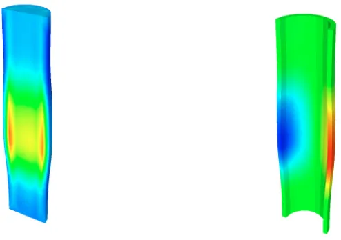
Figure 1. Left: fluid mesh. Right: structure mesh.
The domain used for both simulations is a cylindrical tube of length L3d = 5 along the z axis, with a circular basis of radius at restR0 = 0.5. A relatively coarse mesh was chosen for the simulation, as shown at Figure 1: the mesh is made of 30720 tetrahedra for the structural mesh and 68160 for the fluid mesh. The initial mesh is unstructured in the Oxy plane, but all nodes are contained in one of the 41 sections at altitude
z=i×L3d/40, i= 0,1, . . . ,40.
The wall densityρw was taken equal to 1.2 and the Poisson coefficientνwequal to 0.3. Two different values of the Young modulus E and the wall thickness at rest h0,w were used. For the first simulation, E1 = 3.E6
andh10,w = 0.05, whereas for the second one E2 = 4.E6 and h20,w = 0.1. The density of the fluid chosen was
ρf = 1.0 and its viscosityνf = 0.03.
The temporal discretization used was quite fine (dt= 1E−4) in order to obtain a sufficient amount of data for the optimization. The number of timesteps computed was 99 for the first simulation and 79 for the second one. The simulations were stopped once the pressure wave arrived at the end of the tube, in order to avoid unphysiological reflexion.
The data obtained from each simulation was post-processed in order to have, at each time step and at each section of the tube, the values of the area Ad, the flux Qd and the pressure P d of the blood flow (see the notations in section 3.1.4).
Figure 2. Solution of the 3-d model at time t = 50E−4 for a Young modulus E1 = 4E6.
Left: fluid velocity along thez axis. Right: displacement of the structure alongy axis.
Figure 3. Solution of the 3-d model at time t = 50E−4 for a Young modulus E1 = 6E6.
Left: fluid velocity along thez axis. Right: displacement of the structure alongy axis.
One notes the effect when one increases the Young modulus: the pressure wave is extended in space and decreased in amplitude.
4.2.
Solving the 1-d-model
In order to find the optimal value of a parameter, the algorithm does a series of simulations of the direct 1-d model.
The parameter estimated here wasβ(= β0
2ρA0); all other parameters were kept constant: β1 = 1/2, α= 1,
The 1-d domain, denoted by Ω, was chosen to be slightly shorter than the cylindrical tube used for the 3-d simulations: Ω = [0.5,4.5], and its length was therefore L= 4. This was done in order to avoid the problems arising from the difference in the type of the boundary conditions between the 3-d and the 1-d models.
The 1-d computations were made with a spatial discretization of N = 128 elements of constant length
L/N = 4/128, and a time step dt = 1.e−5, that is ten times smaller than the 3-d time step. These values ensure the Courant condition to be always respected.
4.3.
Measurement operator and cost function
For each test case, a series of estimations ofβ was done using different amounts of data. This means that the measurement operator used for the optimization was changed, and so was, consequently, the expression of the cost function J.
As explained in section 3.1.2, the measurement operator is a weighted sampling of the direct solution expressed by (26). The weights used here were wA≡1 andwQ≡0.1 for all measures. They were chosen to compensate the orders of magnitude of the area (O(1)) and the flux (O(10)) in the vessel. Three different space samplings were chosen: the first one uses 33 measures taken atζj = 0.5 +j×(4/32), for j = 0, . . . ,32. The second one uses 3 measures, at ζ1 = 0.5,ζ2 = 2.5 andζ3= 4.5, and the last one only two, at ζ1 = 0.5 andζ2= 4.5. The time sampling consists in using the data at either all the instants available or only at every ten of them. For the first simulation, that means the measures are taken atθν =ν×dtforν= 0, . . . ,99, or atθν= 10ν×dtfor
ν= 0, . . . ,9. For the second simulation, they are taken atθν =ν×dtforν= 0, . . . ,79 or atθν = 10ν×dt for
ν= 0, . . . ,7.
Let us note that the cost function minimized during each estimation is normalized. Its expression is the following (cf. (29)):
J(β) =
Vt
ν=0
Vz
j=0 Adνj −Aφφzt((νj)) 2
+ (0.1)2
Qdν
j −Qφφtz((νj))
2
Vt
ν=0
Vz
j=0
(Adν
j)2+ (0.1)2(Qdνj)2
.
4.4.
Validating the computation of the cost function gradient
In order to validate the computation of the cost function gradient using the method presented here, its value was compared with the value obtained with the finite difference method. This method consists in computing an approximation of the derivative of the cost functionJ(β) with respect toβ, that is:
∂J
∂β(β) = limh→0
J(β+h)−J(β)
h (45)
The cost function gradient was computed in some test cases with both methods and the results, made in double precision, showed 6 to 7 identical numbers.
4.5.
Expected results of the estimation
Let us recall the role of the parameterβ. As exposed in section 2, to derive the 1-d blood model from the 3-d one, a wall displacement law (cf. (4)) is used, that introduces two positive real parametersβ0 andβ1. In these tests, the power coefficientβ1 is taken equal to 1/2 and the law is reformulated into the expression (6), that only involves one positive parameterβ.
A linear elastic law provides the following expression for β:
β3d=
√ πh0,wE
whereE, h0,w andνw are the wall Young modulus, the wall thickness at rest and the Poisson coefficientused to compute the 3-d data.
The optimal value ofβ, minimizing the difference between the results of the 1-d and 3-d models, is therefore expected to be β3d. It will be shown that this is not the case: the results obtained computing the 1-d model with the estimated optimal value, βestim, fit better to the 3d data than the results obtained with β3d. The accuracy of the estimation algorithm is therefore not to be evaluated from the accuracy on β, but from the accuracy on the error between the 1-d results and the data.
4.6.
Test case 1: shell structure,
E
= 3
.E
6
and
h
0,w= 0
.
05
The first test was made using the 3-d data obtained with a shell / Navier-Stokes coupling. The structure has a Young modulus equal to 3.E6 and a wall thickness equal to 0.05. The number of iterations needed for the optimization varied between 6 and 10 for all the different estimations.
4.6.1. Results of the optimization
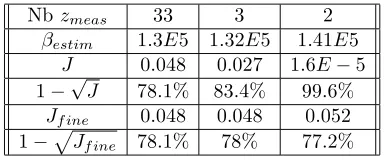
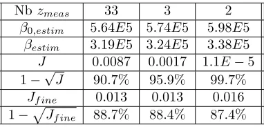
The results obtained are shown in tables 1 and 2: for each estimation, the optimal valueβestim is given, as well as the corresponding value of the minimized cost functionJ and the value 1−√J, that gives the order of explained data.
In order to better compare the precision of the different estimations, we also give the value of a general cost function, called “fine cost function”, and denoted byJf ine. This functionJf inecomputes the least squares error between the 3-d data measured at each of the 99 timesteps and the 33 sections, and the 1-d data obtained with the estimated valueβestim.
Nb zmeas 33 3 2
βestim 1.3E5 1.32E5 1.41E5
J 0.048 0.027 1.6E−5 1−√J 78.1% 83.4% 99.6%
Jf ine 0.048 0.048 0.052 1−Jf ine 78.1% 78% 77.2%
Table 1. Results using 99 time measurements and 33, 3 or 2 spatial measurements for a 3-d
data such that: E= 3E6 andh0,w= 0.05.
Nb zmeas 33 3 2
βestim 1.32E5 1.33E5 1.41E5
J 0.038 0.02 3E−6 1−√J 80.6% 85.9% 99.8%
Jf ine 0.048 0.048 0.052 1−Jf ine 78.0% 78.0% 77.2%
Table 2. Results using 9 time measurements and 33, 3 or 2 spatial measurements for a 3-d
We can see that, logically, the most accurate estimation is obtained in the case where the biggest amount of 3-d data is used for the optimization. But the results do not degenerate too much when the number of time or space measurements is reduced. In fact, the value ofβ estimated from only 9 time and 2 space measurements, provides results that explain 77,2% of the data.
The results are actually quite stable with respect to the amount of data used. Particularly, when the number of time measures varies from 99 to 9, the estimated value ofβ remains almost constant. On the other hand, we notice that the value ofβestim is more sensitive to the variation of the number of space measures. But this sensitivity remains relatively low, the maximal variation of βestim being of 10%, when the amount of space measurements changes from 33 to 2.
4.6.2. Results of the 1-d model using the estimated value βestim
For this test case, the expected value ofβ, according to relation (46), isβ3d= 1.87E5. In order to compare this value with the results of the different estimations, the 1-d model has also been computed usingβ3d. The percentage of explained data obtained with this simulation, measured with the function 1−Jf ine, is of 64%, which is far bellow the one obtained with the different estimations made (see tables 1 and 2).
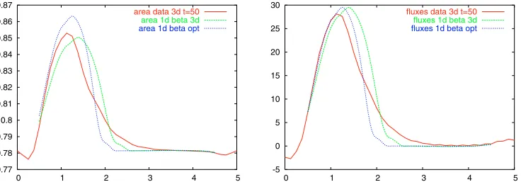
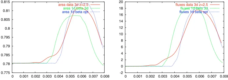
We show next the results of the 1-d model computed using the estimated valueβestim = 1.30E5, obtained from 99 time and 33 space measurements of the 3-d data. The results are compared with the 3-d data and with the 1-d results computed usingβ3d. Note that there is a difference of about 30% between the valuesβestim and
β3d. Figures 4 and 5 represent the area of the vessel and the flux of the blood flow in the whole domain, after 50 and 90 time steps. Figure 6 shows the time evolution of the area and the flux at the middle of the tube, that is at z=L/2.
0.77 0.78 0.79 0.8 0.81 0.82 0.83 0.84 0.85 0.86 0.87
0 1 2 3 4 5 area data 3d t=50
area 1d beta 3d
area 1d beta opt
-5 0 5 10 15 20 25 30
0 1 2 3 4 5 fluxes data 3d t=50
fluxes 1d beta 3d
fluxes 1d beta opt
Figure 4. Area and flux obtained from the 1-d model usingβestim (blue dotted line) andβ3d
(green dashed line), compared to the 3-d data (red line), after 50 timesteps.
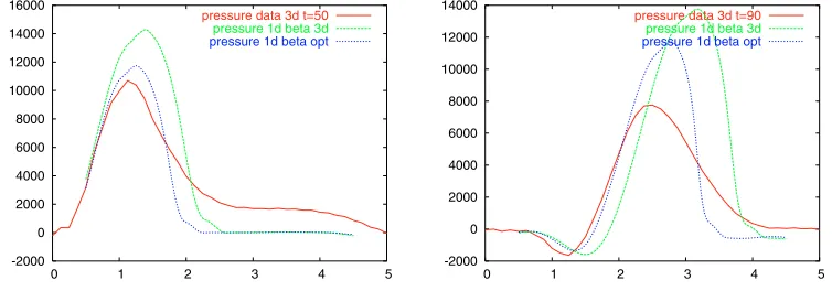
As an additional information, the pressure of the blood flow was computed from the 1-d results according to the wall displacement law (6). It is displayed after 50 and 90 time steps in Figure 7.
On these figures, we observe that the results of the 1-d model manage to capture quite well the phase of the waves of the 3-d data, but not its shape and amplitude. Particularly, the waves of the 3-d data are significantly larger. This can be explained by one of the assumptions made for the derivation of the 1-d model, that considers the vessel as a sequence of independent rings. On the contrary, the 3-d model used to compute the data takes into account the propagation in the structure. On the other hand, the difference in the amplitude can be due to the more important diffusivity of the 3-d models.
0.76 0.77 0.78 0.79 0.8 0.81 0.82 0.83 0.84 0.85 0.86 0.87
0 1 2 3 4 5 area data 3d t=90
area 1d beta 3d
area 1d beta opt
-5 0 5 10 15 20 25 30 35
0 1 2 3 4 5 fluxes data 3d t=90
fluxes 1d beta 3d
fluxes 1d beta opt
Figure 5. Area and flux obtained from the 1-d model usingβestim (blue dotted line) andβ3d
(green dashed line), compared to the 3-d data (red line), after 90 timesteps.
0.78 0.79 0.8 0.81 0.82 0.83 0.84 0.85 0.86 0.87
0 0.001 0.002 0.003 0.004 0.005 0.006 0.007 0.008 0.009 0.01 area data 3d z=2.5
area 1d beta 3d
area 1d beta opt
-5 0 5 10 15 20 25 30
0 0.001 0.002 0.003 0.004 0.005 0.006 0.007 0.008 0.009 0.01 fluxes data 3d z=2.5
fluxes 1d beta 3d
fluxes 1d beta opt
Figure 6. Area and flux obtained from the 1-d model usingβestim (blue dotted line) andβ3d
(green dashed line), compared to the 3-d data (red line), atz=L/2.
-2000 0 2000 4000 6000 8000 10000 12000 14000 16000
0 1 2 3 4 5 pressure data 3d t=50
pressure 1d beta 3d
pressure 1d beta opt
-2000 0 2000 4000 6000 8000 10000 12000 14000
0 1 2 3 4 5 pressure data 3d t=90
pressure 1d beta 3d
pressure 1d beta opt
Figure 7. Pressure obtained from the 1-d model usingβestim(blue dotted line) andβ3d(green
dashed line), compared to the 3-d data (red line). Left: after 50 timesteps. Right: after 90 timesteps.