A Novel Wireless Sensor Node Positioning Algorithm Based on Ant Colony Optimization Algorithm and Neural Network

A Novel Wireless Sensor Node Positioning Algorithm

Based on Ant Colony Optimization Algorithm and

Neural Network

Beichen Chen

Institute of Chemical Technology, Jilin, Jilin, China Northeastern University, Shenyang, Liaoning, China

[email protected]

Abstract—This paper aims to enhance the positioning accuracy of wireless sensor network (WSN) nodes. For this purpose, a WSN node positioning algorithm was proposed based on artificial bee colony (ABC) algorithm and the neural network (NN). First, the parameters between three anchor nodes and the target node were measured. Then, the ABC and NN were introduced to simulate and predict the ranging error, and the weight was determined according to the results. In the proposed algorithm, the cluster structure was effectively combined with the NN model. The weight of backpropagation NN was optimized by the ant colony optimization (ACO) algorithm. Then, the ACO-optimized NN was used to fuse the data collected by WSN nodes. The simulation results show that the proposed algorithm can improve the positioning accuracy of WSN nodes and reduce the time of the search. The research findings shed new light on the positioning of WSN nodes.

Keywords—Wireless sensor network (WSN), neural network (NN), ant colony optimization (ACO) algorithm, data fusion, feature extraction.

1

Introduction

1.1 Wireless sensor network (WSN)

The WSN has been successfully applied in such field as smart home, indoor positioning and environment monitoring, due to its integration of computer, radio and communication technologies. The effect of WSN applications lies in node positioning accuracy, which is affected by many external factors, such as walls, walking bodies and other obstacles. Therefore, it is a focal point in WSN research to improve node positioning [1~3].

type of algorithms. Thus, the range-based algorithms feature a high cost of node positioning, and a narrow scope of application [5~7]. Compared with range-based algorithms, the range-free algorithms are simple, accuracy and widely used [8]. This type of algorithms estimate internodal distance against the intensity of the transmitted signal and then calculate the target node position by trilateration.

In node positioning, the intensity of the received signal is usually determined by range-based algorithms. It is inevitable that the signal intensity would be disturbed by noises like airflow and multipath. In this case, there might be a certain time variation in the intensity of the received signal, which may cause a huge positioning error of sensor nodes [9]. To solve the problem, some experts have improved the conventional received signal intensity positioning algorithm, aiming to eliminate the external noises and enhance the positioning accuracy [10].

In WSN applications, the field data are collected constantly by sensors. The collected data share two common features: the data acquired by the same node remain basically the same within a certain period of time; the data acquired by neighbouring nodes are similar within a short period of time. Thus, the collected data are obviously redundant [11]. To eliminant redundancy, the data fusion technique should be introduced to the WSN to process and retransmit the original data as necessary. This is a good way to reduce the transmission load, lower energy consumption of nodes and prolong the service life of the WSN [12].

1.2 Neural network (NN)

Inspired by the nervous system in human brain, the NN is a adaptive and self-organized model containing numerous interconnected units called neurons. The model is known for its strong self-learning, distributed storage and data processing abilities. Over the years, the NN has been widely adopted to tackle fuzzy information problems that simultaneously involve many factors. The previous studies have shown that the NN is an ideal tool to deal with data fusion in the WSN [13].

Recent years has seen the integration between the NN and ant colony optimization (ACO) algorithm. For instance, Reference [14] introduces the ACO algorithm into the NN, forming an ACO-NN blind equalization algorithm. Reference [15] developed an improved power-efficient gathering in sensor information system (PEGASIS) based on the NN and the ACO algorithm.

1.3 Thesis statement

2

NN and ABC Algorithm

2.1 Backpropagation NN (BPNN)

Let x(i) be the input data. Then, the hidden layer input and output of the BPNN can be expressed as:

(1)

(2)

where 𝜔𝜔"# are the weights of input and hidden layers; 𝜃𝜃# is the corresponding

threshold. Besides, the input and output of the output layer can be expressed as:

(3)

(4)

Where 𝑣𝑣_& are the weights of the hidden and output layers; 𝛾𝛾 is the corresponding threshold.

2.2 ABC algorithm

The ABC algorithm is an optimization technique that simulates the foraging behaviour of honey bees. In the ABC model, the colony consists of three groups of bees: employed bees, onlookers and scouts. It is assumed that there is only one artificial employed bee for each food source. Employed bees go to their food source and come back to hive and dance on this area. The employed bee whose food source has been abandoned becomes a scout and starts to search for finding a new food source. Onlookers watch the dances of employed bees and choose food sources depending on dances.

Let be a collection of n food sources, and 𝑋𝑋_𝑖𝑖 = [𝑥𝑥𝑖𝑖1, 𝑥𝑥𝑖𝑖2, ⋯ , 𝑥𝑥𝑖𝑖𝑖𝑖]𝑇𝑇, 𝑖𝑖 = 1,2, ⋯ , 𝑛𝑛

be the location of food source i, i.e. solution i. Then, the food source can be estimated by the following fitness function:

å

=

-=

i ij j

j

x

i

1

)

(

S

w

q

)

exp(

1

1

b

1 j

n

i ij

j

q

w

-+

=

å

=

j p

j ij j

b

L

=

å

w

-

q

=1

)

exp(

1

1

1 1

g

-+

=

å

=

+ p

i j j

i

(5)

where 𝑓𝑓6 is the objective function value of solution i.

Then, the location of the food source i can be generated randomly.

(6)

where rand (0,1) is a random number

Next, the employed bee’s neighbourhood search for food sources can be expressed as:

(7)

where 𝑣𝑣_6& are the locations of food sources around 𝑥𝑥_6&; and 𝑟𝑟6& is a random number

within (-1, 1).

If a better food source is discovered, the location of the old food source will be replaced with the location of the new one. Otherwise, the location of the old food source will be retained. After the search by all employed bees, the information on food source will be transmitted to the onlookers.

According to fitness values, the onlooker chooses an employed bee to follow at the probability of 𝑃𝑃₆:

(8)

Then, each onlooker searches the neighbourhood for food source and choose better food sources for preservation.

If the food source is not updated after a cycle, the location will be abandoned, and the employed bee will be transformed into a scout and look for a food source according to equation (6).

3

WSN Node Positioning through ABC-Optimized NN

3.1 Trilateration algorithm

In geometry, trilateration is the process of determining the position of a node by its distances from three anchor nodes, using the geometry circles, spheres or triangles. The basic idea of trilateration algorithm is as follows: in 2D geometry, it is known that if a node lies on two circles, then the circle centres, i.e. the anchor nodes, and the two radii

ï

ï

î

ïï

í

ì

<

+

>

+

=

0

,

1

1

0

,

1

1

i i

i i i

f

f

f

f

fit

) )(

1 , 0

( max min

minj j j

j

i x rand x x

x = +

-)

( ij kj

ij ij

ij x r x x

v = +

-å

=

=

i i

i i

fit

fit

P

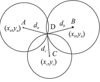
provide sufficient information to narrow the possible locations down to two. An additional circle that passes through the node may narrow the possibilities down to one unique location [17]. The principle of trilateration algorithm is shown in Figure 1 below.

Fig. 1. Principle of trilateration algorithm

As shown in Figure 1, node D is the point to be positioned. Let us denote its coordinates as (𝑥𝑥, 𝑦𝑦). Meanwhile, the positions of the three anchor nodes A, B and C are (xA, yA), (xB, yB) and (xC, yC), respectively, and their distances to node D are dA, dB and dC, respectively. Then, the following relationships can be established:

(9)

3.2 Principle of WSN node positioning through ABC optimized-NN

Let n be the dissipation coefficient of path propagation. Under normal conditions, the received signal strength indicator (RSSI) can be calculated as:

(10)

where A is the ideal value of the RSSI. Equation (10) can be modified as:

(11)

In actual practice, the values of A and n are variable depending on the environment, and often determined empirically by experts. The subjective determination may cause

ï

î

ï

í

ì

=

-+

-=

-+

-=

-+

-2 2 2

2 2 2

2 2 2

)

(

)

(

)

(

)

(

)

(

)

(

C C

C

B B

B

A A

A

d

y

y

x

x

d

y

y

x

x

d

y

y

x

x

)

lg

10

(

n

d

A

RSSI

=

-

+

n

A

RSSI

d

10

)

(

10

-

a huge error to node positioning. To overcome the problem, the values of A and n here are estimated in real time. The estimation process is as follows. The received signal strength indices between anchor node C and anchor nodes A and B can be obtained as:

(12)

Both 𝑑𝑑= and 𝑑𝑑> are Euclidean distances, which can be expressed as:

(13)

The values of A and n can be estimated according to equation (13), offering an accurate depiction of the environment state of the nodes.

To sum up, the WSN node positioning through ABC optimized-NN is implemented in four steps: first, the values of A and n are estimated; second, the NN is introduced to correct the estimated distances; third, the connection weights and thresholds of the NN are optimized by the ABC algorithm to obtain the distance weights; fourth, the location of the target node is calculated by the trilateration algorithm.

3.3 Error correction

The previous studies have shown that the RSSI estimation error increases with the distance of signal transmission. Hence, proper adjustment of distance is needed before estimating the values of A and n, that is, the values should be weighted to reduce the distance error. Weight describes the impact of an anchor node on the target node, while distance reflects the relative position between these two kinds of nodes. Here, weight ω" is defined as

(14)

Where 𝑑𝑑6is a sequence of measured distances between anchor nodes and the target

node. The position of the target node can be expressed as:

(15)

In actual practice, there is always a range error of ∆E. The relationship between actual distance (𝑑𝑑) and measured distance (𝑑𝑑B_{) is:}

(16)

î

í

ì

+

-=

+

-=

)

lg

10

(

RSSI

)

lg

10

(

RSSI

A

d

n

A

d

n

ïî

ï

í

ì

-+

-=

-+

-=

)

(

)

(

)

(

)

(

y

y

x

x

d

y

y

x

x

d

å

-=

d

d

w

å

=

)

,

(

)

,

(

i i i i

Here, the NN is introduced to predict and correct the ranging error, and then the ABC algorithm is employed to optimize the NN parameters; the distance error was estimated by equation (11) and the prediction error is denoted as △_{E’. Thus, we have the}

positioning error correction equation:

(17) During the NN-prediction of positioning error, the error of measured distance was determined by connection weights and thresholds. These weight and thresholds were optimized by the ABC algorithm. The NN predicts the distance error in the following steps:

Step 1 Collect and normalize the sequence of measured distances:

(18)

Step 2 Initialize the parameters, including the number of food sources, the number of iterations, the limit of the control parameter, and the restricted interval of the solution.

Step 3 Initialize the locations of the food sources: 𝑋𝑋𝑖𝑖= [𝑥𝑥𝑖𝑖1, 𝑥𝑥𝑖𝑖2, ⋯ , 𝑥𝑥𝑖𝑖𝑖𝑖]𝑇𝑇, 𝑖𝑖 =

1,2, ⋯ , 𝑛𝑛, with being the number of food sources, and D being the dimension. The dimension can be determined as:

(19) where M, H and N are the number of nodes in the input layer, hidden layer and output layer, respectively.

Step 4 Assign the weights and thresholds of the NN according to the 𝑋𝑋6 position.

Then, the objective function value of 𝑋𝑋₆ can be obtained through learning the training samples:

(20)

Where 𝑑𝑑₆ and 𝑡𝑡_D are actual outputs and expected outputs, respectively; k is the number of training samples.

Step 5 Calculate the fitness value of the new solution 𝑉𝑉₆ around 𝑋𝑋₆ generated by the employed bees. According to the greedy criterion, preserve the one with better fitness between the new and old solutions.

Step 6 Select the solution by the probability of 𝑃𝑃₆. For any new solution 𝑉𝑉₆ generated around 𝑋𝑋₆, retrain the optimal solution in the same way.

Step 7 Abandon the solution if it is not improved after a cycle. In this case, the employed bee will be transformed into a scout and look for a new solution.

Step 8 Find the best solution according to fitness value.

Step 9 After reaching the termination condition, obtain the optimal weights and thresholds of the NN according to the optimal solution; otherwise, return to Step 5.

E d

d¢¢= ¢+D ¢

min max

max

ˆ

y

y

y

y

y

i

-=

n

N H N H H M

D= * + * + +

åå

= =

-=

i m

k i k

t

d

n

fit

1 1

2

Step 10 Relearn the training samples according to the optimal weights and thresholds and establish the ranging error prediction model.

Step 11 Correct the ranging error based on the result of error prediction.

4

Two-Level Data Fusion Algorithm Based on NN

4.1 Two-level data fusion

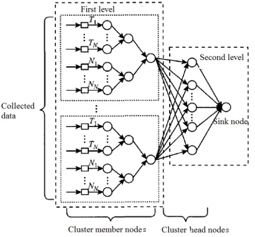
In this research, the data collected by each WSN sensor are subjected to the data fusion by a level data fusion algorithm. Figure 2 illustrates the structure of the two-level data fusion algorithm. As its name suggests, this algorithm adopts a two-two-level NN model. The first level targets the cluster member nodes, while the second level targets the cluster head nodes.

Fig. 2. Structure of the two-level data fusion algorithm

the eigenvalues outputted from the first level as the inputs. The results of the second level will be transferred to the sink node.

4.2 Introduction of ACO algorithm

Based on the previous research results, the ACO algorithm was introduced to the NN. To prevent the trap of local optimum, the heuristic factor was adjusted and search hotspot was set before the ants select the next search path. These moves ensure that the ants will choose the shortest path, thus improving the efficiency of ant colony search.

(1) Adjusting the heuristic factor

In traditional ACO algorithm, 1 d⁄ "#is generally used as the heuristic factor, with d"#

being the distance between city i and city j. This factor ensures that the ants will choose the shortest path during the selection of the next search path. However, the distance relationship η"#(t) = 1 d⁄ "# between city i and city j only reflects the relative location

between the two city nodes, failing to describe the relationship between each node and the starting node. To solve the defect, the heuristic factor can be adjusted as:

q (21)

where d_"# is the distance between the starting node and the current node. The value of d"# is negatively correlated with the probability for the ants to choose the shortest

path. The adjustment considers both the inter-nodal distance and the distance between each node and the starting node, and guides the search towards the global optimal solution.

(2) Setting search hotspots

The shortest path is most likely to fall within the circular search area whose diameter is the distance between the starting node and the target node. Therefore, this area is defined as the area of search hotspots, or the hotspot area. After determining whether the current path is in the hotspot area, it is possible to determine the probability formula for selecting the next path is determined according to whether hotspots are searched. Suppose there are 𝑘𝑘(𝑘𝑘 = 1,2, ⋯ , 𝑆𝑆) ants. Then, the probability for each ant to choose an element in each set of 𝑅𝑅_M6(1 ≤ 𝑖𝑖 ≤ 𝑚𝑚) can be expressed as:

(22)

where 𝜏𝜏6& is the pheromone between i and j; 𝑈𝑈(𝑘𝑘) is the set of cities that the ants

have not visited at the moment; 𝜑𝜑_6&(𝑡𝑡) has different values depending on whether path between i and j falls in the hotspot area:

)

(

1

)

(

ij oj

ij

t

=

d

•

d

h

P

ï

î

ï

í

ì

Ï

Î

=

å

Î

)

(

,

0

)

(

,

)

(

)

(

)

(

)

(

)

(

k

U

j

k

U

j

t

t

t

t

t

P

k U

j ij ij

ij ij ij k

ij a b

b a

h

t

j

h

t

(23)

The introduction of hotspot area helps prevent the local optimum trap and enhance the search efficiency of the ACO algorithm.

5

Simulation Experiments

It is assumed that 100 commonnodes and 20 anchor nodes are randomly distributed in a 2D area (100m×100m). Then, simulation experiments were carried out on Matlab using the proposed algorithm. Let d be the inter-nodal distance. Then, the energy to receive and transmit 1 bit of data can be expressed as:

(24)

(25)

where 𝑑𝑑S is the distance threshold for data transmission.

Next, the node positioning error, an evaluation criterion, can be defined as:

(26)

where (𝑥𝑥, 𝑦𝑦) is the estimated position; (𝑥𝑥B_{, 𝑦𝑦}B_{) is the actual position.}

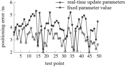
Fig. 3. Effect of real-time updates of A and n on the positioning of sensor nodes

To disclose effect of real-time updates of A and n on the positioning of sensor nodes, the results were compared with those of the fixed parameter value method and the ranging error was determined (Figure 3). As shown in Figure 3, the positioning error after the dynamic updates was smaller than that of the fixed parameter value method,

î

í

ì

£

>

=

area

search

the

in

fall

not

does

)

,

(

,

1

area

search

hot

the

in

falls

)

,

(

,

1

)

(

j

i

j

i

t

j

ïî

ï

í

ì

>

+

£

+

=

,

,

)

,

(

d

d

d

k

kE

d

d

d

k

kE

d

k

E

e

e

RX

k

d

kE

E

(

,

)

=

2

2

(

)

)

(

x

-

x

¢

+

y

-

y

¢

=

indicating that the real-time updates of A and n can accurately describe the state change of sensor nodes.

Fig. 4. Effect of ABC-optimized NN on the positioning of sensor nodes

To verify the effect of ABC-optimized NN, the positioning results of the method were contrasted with those of the positioning method without error correction. According to the results in Figure 4, it is clear that the positioning error of sensor nodes and its range were significantly reduced after the correction by ABC-optimized NN. This means the error correction can prevent the interferences in node positioning, yielding credible positioning results.

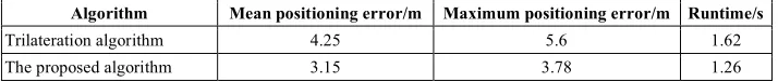
Next, the proposed algorithm was compared with the trilateration algorithm in terms of runtime, mean positioning error and maximum positioning error. The results are listed in Table 1 below.

Table 1. Comparison between the proposed algorithm and the trilateration algorithm Algorithm Mean positioning error/m Maximum positioning error/m Runtime/s

Trilateration algorithm 4.25 5.6 1.62

The proposed algorithm 3.15 3.78 1.26

As shown in Table 1, the trilateration algorithm had a greater mean positioning error, which is mainly caused by the neglection of the external influences. Overall, the proposed algorithm boasts an obviously better positioning effect than trilateration algorithm, as evidenced by the low mean and maximum positioning errors and the short runtime. The good performance is attributable to the real-time updates of the values of A and n and the correction of positioning error by the NN.

6

Conclusions

experiments. The results show that the proposed algorithm can improve the positioning accuracy of WSN nodes and reduce the time of the search. The research findings shed new light on the positioning of WSN nodes.

7

Acknowledgment

This work is supported in part by the Natural Science Foundation of Jilin (Grant No. 20180101336JC), outstanding youth fund of Jilin City Science and Technology Bureau (Grant No. 20166019).

8

References

[1]Zhu, H. S., Sun, L. M. (2009). Development status of wireless sensor network. ZTE Communications, 15(5): 1-5.

[2]Yick, J., Mukherjee, B., Ghosal, D. (2012). Wireless sensor network survey. Computer Networks, 52 (12): 2292-2330. https://doi.org/10.1016/j.comnet.2008.04.002

[3]Garg, V., Jhamb, M. (2013). A review of wireless sensor network on localization technique. International Journal of Engineering Trends and Technology, 4(4): 1049-1053.

[4]Chaurasiya, V. K., Jain, N., Nandi, G. C. (2014). A novel distance estimation approach for 3D localization in wireless sensor network using multidimensional scaling. Information Fusion, 15(1): 5-18. https://doi.org/10.1016/j.inffus.2013.06.003

[5]Priyadarshini, K. J., Ganesh, A. B. (2012). Improvisation of localization algorithm for wireless sensor networks. Procedia Engineering, 38(6): 1186-1191. https://doi.org/10.1016/ j.proeng.2012.06.150

[6]Zhao, J. J., Zhao, Q. W., Li, Z. H., Liu, Y. (2013). An improved weighted centroid localization algorithm based on difference of estimated distances for wireless sensor networks. Telecommunication Systems, 53(1): 25-31. https://doi.org/10.1007/s11235-013-9673-6

[7]Tian, H., Li, C., Xie, J., Liang, Y. (2016). Node localization algorithm for WSN based on time sequence Monte Carlo. Chinese Journal of Sensors and Actuators, 29(11): 1724-1731. [8]Xia, S., Zhu, X., Zou, J. (2015). The improved DV-Hop algorithm based on hop count. Chinese Journal of Sensors and Actuators, 28(5): 757-762. https://doi.org10.3969/j.issn. 1004-1699.2015.05.024

[9]Li, J., Wang, W., Jie, J. (2016). Localization algorithm for wireless sensor networks based on MDSMAP integrated with maximum likelihood estimating. Chine Journal of Sensor and Actuators, 29(4): 572-577.

[10]Cao, S., Wang, Q., Wang, L. (2016). Wireless sensor network node localization based on iterative mechanism of neighborhood rotation and hopping. Computer Engineering, 42(7): 94-99.

[11]Qiu, X. S., Lin, Y. F., Shao, S. J. (2015). Sensor aggregation distribution construction algorithm for smart grid data collection system. Journal of Electronics& Information Technology, 10: 2411-2417.

[13]Hou, X., Zhang, D. W., Zhong, M. Data aggregation of wireless sensor network based on event riven and neural network. Chinese Journal of Sensors and Actuators, 1: 142-148. DOI: 10.3969/j.issn.1004-1699.2014.01.026

[14]Geng, Y., Zhang, L., Sun, Y. (2016). Research on ant colony algorithm optimization neural network Weights blind equalization algorithm. International Journal of Security and Its Applications, 10(2): 95-104. https://doi.org/10.14257/ijsia.2016.10.2.09

[15]Li, T, Ruan, F., Fan, Z. (2015). An improved PEGASIS routing protocol based on neural network and ant colony algorithm. International Journal of Future Generation Communication and Networking, 8(6): 149-160. https://doi.org/10.14257/ijfgcn. 2015.8.6.15

[16]Ni, Z., Li, R., Fang, Q. (2016). Optimization of cloud task scheduling based on discrete artificial bee colony algorithm. Journal of Computer Applications, 36(1): 107-112, 121.

https://doi.org/10.11772/j.issn.1001-9081.2016.01.0107

[17]Liu, S., Huang, J., Liu, H. (2015). An improving DV-Hop algorithm based on multi communication radius. Chinese Journal of Sensors and Actuators, 28(6): 883-887.

9

Authors

Beichen Chen received his Bachelor in Automation and Instrument from Northeastern University, China, in 2003., and his Master degree in Physical Chemistry of Metallurgy from Northeastern University, China in 2007. Currently he is working on Ph.D. Program in Measurement Technology and Automatic Equipment from Northeastern University, China. Meanwhile, he is a lecturer of College of Information and Control Engineering, Jilin Institute of Chemical Technology. His research interests are in sensing technology, Wireless sensor network and embedded system development.