University of Trento University IUAV of Venezia
Yue Feng
A
N
O
PTIMIZATION
I
NDEX TO
I
DENTIFY THE
O
PTIMAL
D
ESIGN
S
OLUTION OF
B
RIDGES
Advisor:
Prof. Enzo Siviero
Università IUAV di Venezia, Venice, Italy
Co-Advisors:
Prof. Baochun Chen, Prof. Bruno Briseghella
Fuzhou University, Fuzhou, China
Prof. Tobia Zordan
Tongji University, Shanghai, China
Prof. Luigi Fenu
University of Cagliari, Cagliari, Italy
UNIVERSITY OF TRENTO
Department of Civil, Environmental and Mechanical Engineering
Final Examination 10 / April / 2014
Board of Examiners
Prof. Maurizio Piazza (Università degli Studi di Trento)
Prof. Andrea Prota (Università degli Studi di Napoli Federico II) Prof. Carmelo Gentile (Politecnico di Milano)
i
SUMMARY
Structural optimization has become an important tool for structural designers, since it allows a better exploitation of material, thus decreasing structure self-weight and saving material costs. Moreover, it helps the designer to find innovative design solutions and structural forms that not only better exploit material but also give the structure higher aesthetic value from an architectural point of view. When applied to real scale structures like bridges, this approach leads to the definition of voids patterns delimiting regions where fluxes of force migrate from force application point to boundary regions and suggests innovative layouts without renouncing to formal and structural aspects. Nevertheless, the criticality of this powerful tool is related to the ease of defining entire families of possible candidate solutions, by modifying input volume reduction ratio to reduce structural weight as much as possible or defining several starting trial solutions based on the judgment of designer. In this case, structural optimization still leads to the best material distribution, but finding the best compromise between material saving and structural performance is a designer choice.
iii
SOMMARIO
L’ottimizzazione strutturale e’ oramai ritenuta essere un importante strumento di supporto ai progettisti in quanto consente di riuscire a sfruttare al meglio il materiale, e in questo modo ottenere una riduzione dei pesi propri e un risparmio nelle quantita’ utilizzate. Inoltre, come dimostrato da varie recenti realizzazioni, puo’ essere di aiuto al progettista nella ricerca di innovative soluzioni progettuali e forme strutturali che coniugano ad un ottimo utilizzo del materiale anche un alto valore estetico. Se applicate nel campo delle grandi strutture e dei ponti, le tecniche di ottimizzazione e in particolare l’otttimizzazione topologica, possono portare alla identificazione di zone con materiale poco sfruttato in funzione del flusso delle forze dal loro punto di applicazione ai vincoli e quindi alla sua succesiva rimozione e alla modifica della forma iniziale e/o alla definizione di cavita’ al suo interno. Tuttavia la criticita’ di questo strumento e’ rappresentata dalla scelta della soluzione progettualmente piu’ idonea all’interno della famiglia delle possibili soluzioni definite dal processo di ottimizzazione, che risulta fortemente influenzata dalla scelta degli input iniziali e dei parametri da ottimizzare.
v
DEDICATION
vii
ACKNOWLEDGEMENTS
Foremost, I would like to express my sincere gratitude to my advisor Prof. Enzo Siviero and Prof. Baochun Chen for the continuous support of my Ph.D study and research during my study in Italy. Their knowledge and expertise have been a precious reference during these three years.
I would like to express my special appreciation and thanks to Prof. Bruno Briseghella and Prof. Tobia Zordan for their great kindest helps and advices not only in my studies but also in my livings, to make this research work possible. They have supported me throughout my thesis with their patience and knowledge whilst provided me the office to work and treated me as a member of their company during these three years.
My sincere thanks also go to Dr. Cheng Lan and Dr. Enrico Mazzarolo for the supports they provided at times of critical need. I appreciate their vast knowledge and skill in structural optimization area, and their assistance in using softwares and writing papers. Some parts of this research are developed on the basis of works done by them.
ix
CONTENTS
CHAPTER 1
1. INTRODUCTION ... 1
1.1.THE ORIGIN OF OPTIMIZATION INDEX ... 1
1.2.EXTENSION OF OPTIMIZATION INDEX... 4
1.3.LAYOUT OF THESIS ... 7
CHAPTER 2 2. STATE-OF-ART: STRUCTURAL OPTIMIZATION ... 9
2.1.PROBLEM FORMULATION ...11
2.2.DESIGN OPTIMIZATION METHODS ...13
2.2.1 Mathematical Programming Techniques ...14
2.2.2 Optimality Criteria Approaches ...16
2.2.3 Heuristic Algorithms ...17
2.2.4 Optimization Problems Using MATLAB ...18
2.3.NUMERICAL METHODS FOR TOPOLOGICAL OPTIMIZATION ...19
2.3.1 Material Interpolation Method...21
2.3.2 Evolutionary Structural Optimization (ESO) Method ...25
2.3.3 Level Set Method ...26
2.3.4 Numerical Instabilities ...27
CHAPTER 3 3. PROPOSED OPTIMIZATION INDEX ...29
3.1.OPTIMUM INDEX FORMULATION FOR SINGLE-FAMILY MULTI-SOLUTIONS ...30
3.2.GENERALIZED VERSION FOR MULTI-FAMILIES MULTI-SOLUTIONS ...34
CHAPTER 4 4. FOOTBRIDGES SUPPORTED BY CONCRETE SHELL ...37
4.1.SHELL-SUPPORTED BRIDGES DESIGN ...39
4.1.1 Shell Form-Finding ...39
4.1.2 Finite Element Model ...40
4.1.3 Choice of Shell Thickness ...42
x
4.2.1 Different Models Considered ... 45
4.2.2 Results of Shell Bridge T_0.15 ... 46
4.2.3 Results of Shell Bridge T_0.20 ... 55
4.2.4 Results of Shell Bridge T_0.32 ... 63
4.3.COMPARISON BETWEEN TENTATIVE MODELS ... 70
CHAPTER 5 5. CALATRAVA BRIDGE OF VENICE ... 77
5.1.CALATRAVA BRIDGE ... 80
5.1.1 General Situation ... 80
5.1.2 Finite Element Model ... 81
5.1.3 Mechanical Behaviour ... 82
5.2.STRUCTURAL OPTIMIZATION ... 84
5.2.1 Different Models Considered ... 84
5.2.2 Optimization Results of Minimizing Total Volume ... 86
5.2.3 Optimization Results of Minimizing Horizontal Force ... 92
5.3.IDENTIFICATION OF THE BEST DESIGN SOLUTION... 99
CHAPTER 6 6. CABLE-STAYED BRIDGES ... 107
6.1.DESIGN OF CABLES ... 108
6.1.1 Cable Force Optimization Methods ... 108
6.1.2 Optimization Problem Description ... 110
6.1.3 Programs Implemented for Optimization ... 111
6.1.4 Optimization Procedure ... 112
6.2.SINGLE CABLE PLANE CABLE-STAYED BRIDGE ... 113
6.2.1 General Situation ... 113
6.2.2 Finite Element Model ... 115
6.2.3 Cable Area and Initial Force Optimization Results ... 116
6.2.4 Thickness Optimization ... 122
6.2.5 Comparison between Different Models ... 125
6.3.DOUBLE CABLE PLANES CABLE-STAYED BRIDGE ... 127
6.3.1 General Situation ... 127
6.3.2 Finite Element Model ... 129
6.3.3 Cable Area and Cable Force Optimization Results ... 132
6.3.4 Thickness Optimization ... 151
6.3.5 Comparison between Different Models ... 156
CHAPTER 1.INTRODUCTION
1
CHAPTER 1
1. INTRODUCTION
1.1. The Origin of Optimization Index
Structural optimization is the subject of achieving the best performance for a structure with various constraints such as a given amount of material, limitation of peak stress and deflection. Based on strong demand of lightweight, low-cost and high-performance structures due to the limited material resources and technological competition, optimal structure design is becoming increasingly important (Huang and Xie, 2010) and attracting considerable attention (Banichuk and Neittaanmäki, 2010). Benefit from the availability of high-speed computers and the rapid improvements in algorithms, the structural optimization is rapidly becoming an integral part of the structure design process and as an important tool for designers in the last decades (Huang and Xie, 2009).
Structural optimization can be classified into three categories, namely sizing, shape, and topology optimization, each of them address different aspect of the structural design problem (Christensen and Klarbring, 2009). Sizing optimization is to find the optimal design by changing the size variables such as cross-sectional dimensions of trussed and frames, or the thicknesses of plates (Huang and Xie, 2010). Shape optimization is to find the optimum shape of a domain which defined as design variable. Topology optimization of discrete structures is to search for the optimal spatial order and connectivity of the bars in a typical problem, while topology optimization of continuum structures is to find the optimal designs by determining the best number and locations and shape of cavities in the design domain (Bendsoe and Sigmund, 2003, Huang and Xie, 2010).
2
natural frequencies (Achtziger and Kocvara, 2007, Allaire, et al., 2001, Pedersen, 2000).
When applied to a solid or a shell shaped structure, topology optimization leads to the definition of voids patterns delimiting regions where fluxes of force migrate from force application point to boundary regions. If implemented into FE codes and applied to real scale structures like tall buildings, this approach may suggests innovative layouts and provides higher aesthetic value to the investigated structure, without renouncing to formal and structural aspects. Topology optimization results then to be a valid aid for the designer to find the most suitable structural shape not only from an engineering point of view but even an architectural one, leading to a practical connection between the two complementary disciplines.
In addition when topology optimization applied to bridge structures, it allows not only finding a conceptual layout of a design with the lightest and stiffest structure while satisfying certain specified design constraints, but also simplifying the design process and significantly improving efficiency of design. As we known, in the traditional design of bridge structures, bridges are designed based on engineering theories and previous experience, which would involve the preliminary design, structural analysis and check against requirements of mechanical behavior (Guan, et al., 2003). Such a design is followed by design modification, re-analysis and re-checking process and is very expensive and time-consuming. With the topology optimization technique implemented into FE code, the design process can be defined by a set of design variables and constraints as well as objective function and thereby simplified.
Nevertheless, the criticality of this powerful tool is related to the ease of defining entire families of possible candidate solutions, by simply modifying input volume reduction (VR) ratio. Designer could be tempted to reduce structural weight as much as possible. In this case, topology procedure still leads to the best material distribution for the specific target volume, but finding the best compromise between material saving and structural performance is a designer choice.
CHAPTER 1.INTRODUCTION
3 A former formulation for considered GOI was applied to the structural optimization of a steel-concrete arch bridge built is San Donà in the province of Venice, Italy. The bridge was already partially built while the Italian Seismic Code was updated together with a new seismic classification of Italian territory. It prescribed higher acceleration values, requiring a much higher increase of resistance (35%) of the already existing foundations. Hence, seismic retrofitting of this bridge required for a considerable lightening of the superstructure and topological optimization was used to this purpose. Starting from a reference identified solution for the steel deck, consisting in two longitudinal box girder connected by a continuous bottom flange, several candidate solutions were generated from optimization analysis, depending on imposed volume reduction. What is more, although the design objective was the reduction of superstructure weight, the increase in VR causes an increase of both the stress and deflections of bridge, whose control was a competing requirement with respect to VR. Therefore, an issue to identify the best choice among entire candidate solutions is faced and a global optimization index (GOI) defined for this purpose.
Such an index should provide an uncomplicated mathematical procedure for ease application to identify the best design solution, but at the same time has to take into account weight reduction and structural response of candidate solutions. Therefore, two response indexes (RIs) are defined firstly to summarize the overall behavior of the whole structure, namely response index of stress RI(σ) and response index of deformation RI(d). The former is Von Mises stress averaged throughout the whole steel superstructure and was considered as representative of the stress level, whereas the latter is deflection at mid span and was considered as representative of the deformation level.
To take into account the weight reduction, after the introduction of a penalty exponent to the scaling coefficient 1/VR which able to favor design solutions with higher VR, optimization indexes (OIs) of stress and deformation were defined through the comparison of the variation of stress and deformation with respect to the variation of VR, respectively. Eventually, global optimization index (GOI) considering both stress and deformation of structural response was defined by averaging the two
OIs.
4
compromise between material saving and bridge performances, these letters defined in term of stress field and deformations.
1.2. Extension of Optimization Index
However, during earlier designing phases of a project, in particular in the case of spatial shell structures, several starting trial solutions as well as reference solutions might being defined based on the judgment of designer, each solution characterized by a particular layout, material property or distribution of boundary conditions. In this case, topology optimization is still a viable tool to optimize structures, but it would lead to the definition of entire families of possible candidate solutions, depending on input VR target. Therefore, the problem is changed from single-family multi-solutions to multi-families multi-solutions.
To face this particular issue, a further GOI* formulation which based on a further OI*
is presented in this thesis. Proposed global optimization index allows not only to identify best candidate solution originated by a unique reference model, but even comparing structural performances between candidates solution derived by several starting trial solutions.
Same as the index proposed originally, two response indexes (RIs) are defined firstly to summarize the overall behavior of structure, namely response index of stress RI(σ) and response index of deformation RI(d). The former is considered as representative of the stress level, while the latter is considered as representative of the deformation level. However, to extend the applications of OI* to other optimization techniques and bridge structures, according to the structure type and optimization techniques, the stress level can be averaged stress or maximum stress throughout the whole structure, and the deformation level can be deflection at mid span or deflection at tower top.
CHAPTER 1.INTRODUCTION
5 In this thesis, to present to the reader potentially and effectiveness of defined GOI*, three different cases with different structure type or different optimization techniques were studied, namely Optimization of Footbridges Supported By Concrete Shell, Optimization of Calatrava Bridge In Venice and Optimization of Two Cable-stayed Bridges.
In the real case of footbridges supported by concrete shell, the problem related to the tensile stresses rising in concrete shell bridges is faced. When designing bridges supported by a shell in reinforced concrete (RC), it is worth choosing shells with minimal area that, being anticlastic and therefore subject to biaxial compression, well exploited compressive strength of concrete and well prevented cracks propagation. Notwithstanding the use of form-finding algorithms in order to obtain a shell of minimal area subject to biaxial compression, unwished bending moments and related tensile stresses unavoidably arise in some regions of the shell. A previous publication written by the authors (Briseghella, et al., 2013) demonstrated as such unavoidable tensile stresses can be further eliminated by removing material from the shell regions where unwished bending moments arise, thus obtaining a shell structure with voids, by means of topology optimization.
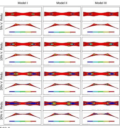
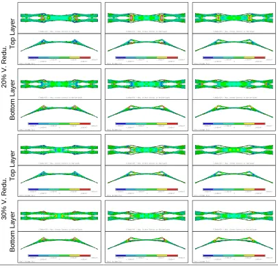
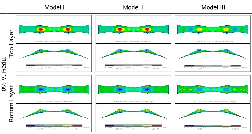
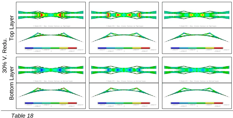
Hence, starting from three footbridges supported by concrete shells with different shape and thicknesses, finite element topological optimization procedures were carried out in order to minimize the volume of the shells of a certain percentage. After identifying the shells regions where the pseudo densities obtained from previous topological optimization results are lower, the geometries of the shells are updated by eliminating the material of these regions. With an iterative procedure of form finding and topological optimization, shells with a pattern of holes are obtained and the areas of shells regions with low tensile stresses are minimized. At the end, the optimum design solutions of three bridges were identified among all the solutions with proposed GOI*.
6
critical aspect considering the soft soil of Venice. Secondly, the open cross-section with π-shaped steel plates and the open truss arch ribs with straight-like web members with no diagonals need not only to withstand shear forces of the main arch, but even local bending moments, leading the stress of some members close to critical state. Besides, being the stiffness of main arch rib relatively small, large bending deformation occurs under asymmetric loading. Finally, the third vibration mode of the main arch is close to the pedestrian step frequency, which is extremely liable to cause the pedestrian and bridge resonance.
Some structural defectiveness mentioned above particularly the occurrence of huge horizontal thrust could be reduced if the bridge with better design such as more reasonable thickness distribution or considering bridge’s abutment deformability. To this aim, three tentative starting models were identified by considering bridge’s abutment deformability through spring-damper elements and introducing tensioning cables along two bottom arches of the bridge, the sizing optimization by means of finite elements of these three models were carried out. Several candidate solutions were obtained due to the different value of elastic stiffness K of spring-damper elements and initial strain
ε
of tensioning cables and their results are used to validate the effectiveness of the proposed GOI*.Cable-stayed bridges are statically indeterminate structures due to its composition. Their structural behavior is the result of a complex interaction between several parameters. The cable arrangement and stiffness distribution in the cables, deck and pylons affected the structural behavior of cable-stayed bridge greatly (Walther, 1999). In the design of cable-stayed bridges, the total number of cables is an important design consideration. It plays an important role not only in the mechanical behavior of bridges but also in aesthetic point of view. Moreover, to get more attractive appearance, sometimes the designer would like to change the angle of the tower.
CHAPTER 1.INTRODUCTION
7 assigned to starting models to carry out thickness optimization of steel plates of bridge deck. Eventually, the results are used to validate the effectiveness of the proposed GOI*.
1.3. Layout of Thesis
Besides this chapter, in the main body of the thesis, it consists of 5 chapters, from Ch.2 to Ch.6 that introduced as following:
Chapter 2, it states a brief development history of optimization techniques and their
applications in structural field, including a general statement of structural optimization problems and the numerical methods of design optimization and topology optimization of continuum structures.
Chapter 3, it presents the optimization index to identify the optimal design solution.
Based on the original index proposed by Bruno Briseghella et al., a generalized formulation was proposed to solve not only the single-family multi-solutions problem but also multi-families multi-solutions problem.
Chapter 4, it presents a case study on footbridges supported by concrete shell. Starting from three footbridges supported by concrete shell, finite element topological optimization procedures were carried out. The geometries of the shells are updated by eliminating the material of shell regions with lower pseudo densities. With an iterative procedure of form finding and topological optimization, shells with a pattern of holes are obtained and the areas of shell regions with low tensile stresses are minimized. At the end, the optimum design solution was identified among all the solutions with proposed index.
Chapter 5, it presents a case study on Calatrava Bridge. Starting from three tentative
models based on the original design, the sizing optimization by means of finite elements of this three models were carried out, the results are used to validate the effectiveness of the proposed optimization index.
Chapter 6, it presents a case study on two cable-stayed bridges. Starting from
8
models to carry out thickness optimization of steel plates of bridge deck and used to validate the effectiveness of the proposed optimization index.
CHAPTER 2.STATE-OF-ART:STRUCTURAL OPTIMIZATION
9
CHAPTER 2
2. STATE-OF-ART: STRUCTURAL OPTIMIZATION
Optimization is a mathematical discipline that concerns with finding minimum and maximum value of some objective functions while subject to so-called constraints (Ding, 1986, Hsu, 1994, Nocedal and Wright, 2006). The beginnings of optimization problems can be traced to the early period of World War II (Elishakoff and Ohsaki, 2010). During that war, the British military faced the problem of allocating very scarce and limited resources to several activities (Rao and Rao, 2009). The methods developed to solve the allocation of limited resources during that period became known as operations research.
The existence of optimization methods can be traced to the days of Newton, Lagrange and Cauchy (Brandt and Wasiutynski, 1963, Ravindran, et al., 2006, Schoofs, 1993). In 1840s, Cauchy made the first application of the steepest descent method to solve unconstrained minimization problems. A long time later in 1947, the development of the simplex method by Dantzig for linear programming methods accelerated the development of methods of constrained optimization (Belegundu and Chandrupatla, 2011, Dantzig, 1998). Following this, the techniques have later grown to be applied to various of scientific and engineering domain (Liang, 2004). Structural optimization is just a traditional and popular subject when the optimization theory applied on structural engineering.
10
In 1960, Schmit (Schmit, 1960) proposed a new approach which has served as an conceptual foundation for the development of many modern structural optimization methods. He introduced an idea of using mathematical programming techniques to solve the nonlinear inequality constrained problem of designing clastic structures under a multiplicity of loading conditions. Prior to that time there were no texts on nonlinear programming.
A few year later, an alternative approach was presented in analytical form by Prager, et al. (Prager and Taylor, 1967), which became popularly known as the ―Optimality Criteria‖ approach. The optimality criteria approach is first to establish the criterion to be satisfy while subject to the constraints. It solves the optimality conditions directly rather than minimize the objective function directly. Although the optimality criteria approach was largely intuitive, its advantage of easily programmed for the computer and relatively independent of problem size make it quite attractive and effective as a design tool.
Since then, the field of structural optimization has experienced many new developments in both computational techniques and applications. In the last decades, based on strong demand of lightweight, low-cost and high-performance structures due to the limited material resources and technological competition, structural optimization with the aim of achieving the best performance for a structure with various constraints is becoming increasingly important, and it has become an important tool for engineering designers benefit from the availability of high-speed computers and the rapid improvements in algorithms (Huang and Xie, 2010).
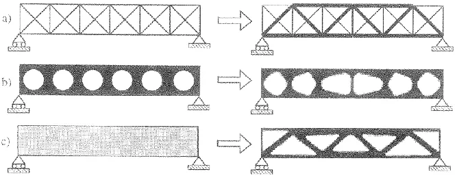
Fig. 1Three categories of structural optimization. a) sizing optimization of a truss structure, b) shape optimization and c) topology optimization (Bendsoe and Sigmund, 2003).
CHAPTER 2.STATE-OF-ART:STRUCTURAL OPTIMIZATION
11 aspect of the structural design problem (Christensen and Klarbring, 2009). Sizing optimization is to find the optimal design by changing the size variables such as cross-sectional dimensions of trussed and frames, or the thicknesses of plates (Huang and Xie, 2010). Shape optimization is to find the optimum shape of a domain which defined as design variable. It is mainly performed on continuum structures by modifying the predetermined boundaries to achieve the optimal designs. Depending on the type of a structure, there are two types of topology optimization, i.e. discrete or continuous. Topology optimization of discrete structures is to search for the optimal spatial order and connectivity of the bars in a typical problem, while topology optimization of continuum structures is to find the optimal designs by determining the number and location and shape of cavities in the design domain (Bendsoe and Sigmund, 2003, Huang and Xie, 2010).
2.1. Problem Formulation
Mathematically speaking, optimization is the minimization or maximization of a function subject to constraints on its variables. It can be simply formulate and written as:
Minimize
f
( )
x
(1)Subject to:
( )
0
1, 2, 3,
,
( )
0
1, 2, 3,
,
x
x
ij
l
i
n
j
m
g
(2)The problem stated above is a constrained optimization problem. The problems are unconstrained optimization problems when there are no any constraints. Here X is the Design Variable (DV) vector,
f
( )
x
is termed the Objective Function (OBJ),( )
x
i
l
andg
j( )
x
are known as equality and inequality constraints, respectively.They are also known as State Variables (SVs) in the optimization procedure. The number of design variables and the number of equality and inequality constraints need not be related in any way.
12
Design Variables are independent quantities, which varied to achieve the optimum design (Roy, et al., 2008). Any structural optimization problem is defined by a set of quantities some of which are viewed as variables during the design process. In general, certain quantities are usually fixed at the outset and these are called pre-assigned parameters. All the other quantities are treated as variables in the design process and are called design variables (Rao and Rao, 2009). The design variables describe the design and can be changed during optimization. It may represent geometry or choice of material. When it describes geometry, it may relate to a sophisticated interpolation of shape or it may simply be the area of a bar, or the thickness of a sheet (Spillers and MacBain, 2009).
State Variables (SVs)
State Variables are quantities that constrain the design. They are also known as "dependent variables" due to they are typically response quantities that are functions of the design variables. In many practical problems, the design variables cannot be chosen arbitrarily but have to satisfy certain specified functional and other requirements. The restrictions that must be satisfied to produce an acceptable design are collectively called design constraints (Rao and Rao, 2009). There are two types of constraints, namely functional constraints and geometric constraints. The latter represent physical limitations on the design variables, while the former represent limitations on the behavior or performance of the system and are state variables. For a given mechanical structure, the state variables usually are the response of the structure in terms of displacement, stress, strain or force.
Objective Function (OBJ)
CHAPTER 2.STATE-OF-ART:STRUCTURAL OPTIMIZATION
13 more than one criterion to be satisfied simultaneously. An optimization problem involving multiple objective functions is known as a multi-objective optimization.
2.2. Design Optimization Methods
The purpose of many structural design problems is to find the optimum design among many possible candidates (Choi and Kim, 2005). An optimum design is the one that as effective as possible, and is the one that meets all specified requirements yet demands a minimum in terms of expenses such as weight, surface area, volume, stress, cost, and other factors in structural engineering. In practical engineering, any aspect of design would be optimized, just like dimensions (such as thickness), shape (such as fillet radii), placement of supports, cost of fabrication, natural frequency, material property, and so on (Ansys, 2007).
The definition of an optimization problem always contains several steps which beginning from identification of design variables and their bounds, then to the identification of constraints and objective function. Immediately following the defining of optimization problem, the algorithms to find the optimum design is the goal of the design optimization problem. There is no single method available for solving all optimization problems efficiently. Hence a number of optimization methods have been developed for solving different types of optimization problems. In the area of structural, there are three main categories optimization methods, namely Mathematical Programming Techniques, Optimality Criteria Approaches and Heuristic Algorithms.
14
Optimality criteria approaches pre-establish criteria to evaluate the structural performance such as stress, strain energy, frequency and etc. based on experience and mechanical engineering concepts, set the Kuhn-Tucker conditions (referred to as KT conditions) as the requirement that optimal solution should satisfy, then the criteria used to optimize the design variables and update the Lagrange multipliers, find the best solution from all the feasible design solutions through an iterative approach at the end. Optimality criteria approaches have an intuitive physical meaning, need not derivative information of function or constraints, less iterations, high speed convergence and high computational efficiency. Furthermore, it is particularly suitable for large scale projects which need a large amount of calculation due to the insensitivity to the increase of the design variables. However, compare to mathematical programming techniques and heuristic algorithms, the optimization always converge to local optima due to the lack of rigorous theoretical foundation. In addition, it is not a general method which can be applied on different optimization problems.
Heuristic algorithms are optimization methods that conceptually different from the traditional mathematical programming techniques. These methods are labeled as modern or nontraditional methods of optimization. Most of these methods are based on certain characteristics and behavior of biological, molecular, swarm of insects, and neurobiological systems. The most rational structures in the world are often created by nature. Bones of animals, plant stems are the formation of a natural evolution and continuous improvement in the long history. Heuristic algorithms are just methods finding the optimal solution in the feasible region when applied to structural optimization according to the laws of nature. In general, although cannot guarantee the final result is global optimal solution, but generally can approach the global optimal solution. Furthermore, the mathematical calculations are not complex, However, a large amount of calculation always needed due to the difficult convergence.
2.2.1 Mathematical Programming Techniques
CHAPTER 2.STATE-OF-ART:STRUCTURAL OPTIMIZATION
15 Dantzig, 1998). In the area of structural, most problems are not linear. However, one way of solving nonlinear programming (NLP) problems is to transform them into a sequence of linear programs (Arora, 2004, Kim, et al., 2002). In addition, some NLP methods solve an LP problem during their iterative solution processes. Thus, linear programming methods are useful in many applications. The standard form of an LP problem with m constraints and n variables can be represented as follows:
minimize
subject to
f
T
c u
Au
b
u
0, b
0
(3)
Where c is the coefficient of the cost function, u is the vector of design variables to be determined, A ism×n matrix, andb is m×1 vector. Inequality constraints can be transformed to equality constraints by introducing slack variables. Linear programming problems are convex problems. Hence, a local minimum is indeed a global minimum.
The simplex method is a very efficient method for solving linear programming problems. The method was developed by George Dantzig (Dantzig, 1998) in 1947 and has been widely used since then. A positive feature of a linear programming problem is that the solution always lies on the boundary of the feasible region. Thus, the simplex method finds a solution by moving each corner point of the convex boundary. Therefore, the basic idea of the simplex method is to proceed from one basic feasible solution to another in a way that continually decreases the cost function until the minimum is reached (Nocedal and Wright, 2006).
16
Based on the nature of design variables encountered, optimization problems can be classified into unconstrained optimization problems or constrained optimization problems. When there are no constraints on the design problem, it is referred to as an unconstrained optimization problem. On the contrary, constrained optimization problem are with constraints. A very common instance of a constrained optimization problem arises in finding the minimum weight design of a structure subject to constraints on stress and deflection. Even if most engineering problems have constraints, these problems can be transformed into unconstrained ones by using the penalty method, or the Lagrange multiplier method.
Direct Methods Indirect Methods
Unconstrained Optimization Problems
Random search method Steepest descent method
Gird search method Fletcher–Reeves method
Univariate method Newton’s method
Pattern search methods Marquardt method
Powell’s method Quasi-Newton methods
Simplex method Conjugate gradient method
Constrained Optimization Problems
Random search methods Transformation of variables technique
Heuristic search methods Sequential unconstrained minimization techniques
Complex method Interior penalty function method
Objective and constraint approximation methods Exterior penalty function method
Sequential linear programming method Augmented Lagrange multiplier method Sequential quadratic programming method
Feasible direction Method Zoutendijk’s method
Gradient projection method Generalized reduced gradient method
Table 1
Methods of nonlinear mathematical optimization problems (Rao and Rao, 2009)
2.2.2 Optimality Criteria Approaches
CHAPTER 2.STATE-OF-ART:STRUCTURAL OPTIMIZATION
17 In general, optimality criteria methods are algorithms that seek the optimum through finding a solution that satisfies some pre-specified criteria which are postulated to correspond to the optimal result for the problem. Among the OC methods, the fully stressed design (FSD) method has a long history. Due to its ease of implementation and fast convergence, it was considered a viable alternative to formal optimization algorithms and widely used. However, it has a main weak point that without a rigorous mathematical basis.
Compared with classical optimization, in which problems are described in terms of objective functions and constraints and then solved using some mathematical programming algorithm, optimality criteria methods analyzed a structure and redesigned it on the basis of some resizing rule. Therefore, while the methods of mathematical programming are formal in the sense of mathematics, optimality criteria methods are considered to be heuristic. In these methods the optimum is sought without explicit concern for an objective function (Groenwold and Etman, 2009, Spillers and MacBain, 2009).
The most important topic in the optimality criteria approach is the concept of scaling. The next two important topics are the iterative algorithm together with the specialization of the Lagrangian multipliers. All of these concepts will be derived as function of the sensitivity derivatives of the constraints and the objective functions. Then this optimization will no longer be addressed in the context of a single discipline, but instead it will be derived in terms of sensitivity derivatives which can be obtained for all disciplines (Venkayya, 1989).
2.2.3 Heuristic Algorithms
18
neural-network-based methods, the problem is modeled as a network consisting of several neurons, and the network is trained suitably to solve the optimization problem efficiently (Rao and Rao, 2009).
Among all the heuristic algorithms, genetic algorithms (GA) have the most in-depth research and widest application. It generates solutions to optimization problems using techniques inspired by natural evolution, such as inheritance, mutation, selection and crossover. In a genetic algorithm, a population of candidate solutions (called individuals, creatures, or phenotypes) to an optimization problem is evolved toward better solutions. The evolution usually starts from a population of randomly generated individuals which is called a generation, and is an iterative process. In each generation, the fitness (usually the value of the objective function in the optimization problem being solved) of every individual in the population is evaluated. The more fit individuals are stochastically selected from the current population, and genome of each individual is modified to form a new generation. The new generation of candidate solutions is then used in the next iteration of the algorithm. Commonly, the algorithm terminates when either a maximum number of generations has been produced, or a satisfactory fitness level has been reached for the population (Madeira, et al., 2009).
Compared with the traditional optimization methods, heuristic algorithms need not the derivative information of the objective function and provide several potential optimal solutions to designers. Moreover, the conversion process of design solutions is random and the operand is a code group contains the design variable information rather than the design variable itself.
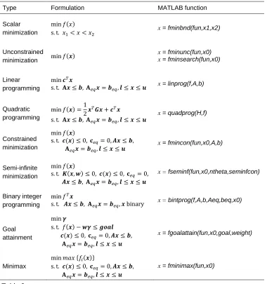
2.2.4 Optimization Problems Using MATLAB
CHAPTER 2.STATE-OF-ART:STRUCTURAL OPTIMIZATION
19 information for using the various programs can be found in the user’s guide for the optimization toolbox.
Type Formulation MATLAB function
Scalar minimization
( )
x = fminbnd(fun,x1,x2)
Unconstrained
minimization ( )
x = fminunc(fun,x0) x = fminsearch(fun,x0)
Linear programming
x = linprog(f,A,b)
Quadratic programming
( )
x = quadprog(H,f)
Constrained minimization
( )
( )
x = fmincon(fun,x0,A,b)
Semi-infinite minimization
( )
( ) ( )
x = fseminf(fun,x0,ntheta,seminfcon)
Binary integer programming
x = bintprog(f,A,b,Aeq,beq,x0)
Goal attainment
( )
( )
x = fgoalattain(fun,x0,goal,weight)
Minimax
* ( )+
( )
x = fminimax(fun,x0)
Table 2
MATLAB programs or functions for solving optimization problems (Guide, 1998)
2.3. Numerical Methods for Topological Optimization
20
optimization stage, it is used for conceptual design, and thus the stage where lightweight can be achieved. In the past three decades, topology optimization has become a powerful and increasingly popular tool for designers and engineers in the early stages of the design process (Bendsoe and Sigmund, 2003, Rahmatalla and Swan, 2003).
Topology optimization is a rapidly expanding research field in structural optimization, its application to bridge structures is being considered as one of the most challenging and committing tasks in structural design. It is a form of "shape" optimization, sometimes referred to as "layout" optimization. The purpose of topology optimization is to find the best use of material for a body such that an objective criterion (such as global stiffness or natural frequency) takes on a maximum/minimum value subject to given constraints (such as volume reduction). The standard formulation of topology optimization defines the problem as minimizing the structural compliance while satisfying a constraint on the volume of the structure (Release, 2007).
Topology optimization is actually the optimization of spatial materials distribution. Its method solves the basic engineering problem of distributing a limited amount of material in a design space. The first paper on topology optimization was published over a century ago by the versatile Australian inventor Michell, who derived optimality criteria for the least weight layout of trusses. In 1976, Prager and Rozvany formulated the first general theory of topology optimization, termed ―optimal layout theory‖. After that, structural topology optimization has been extensively explored, especially for continuum structures (Rozvany, 2008). Many optimization methods such as the Homogenization Technique, Solid Isotropic Material with Penalization (SIMP), Evolutionary Structural Optimization (ESO) and Bi-directional Evolutionary Structural Optimization (BESO) have been developed.
CHAPTER 2.STATE-OF-ART:STRUCTURAL OPTIMIZATION
21 Following the topology optimization of structures characterized by mathematical problems through the numerical methods, suitable mathematical optimization method needs to be selected and applied on the structures. As mentioned above, three main categories mathematical optimization methods are available, namely mathematical programming techniques, optimality criteria approaches and heuristic algorithms. During the optimization procedure, there will be some numerical instability problems with the use of finite element analysis software, such as porous, checkerboard, mesh dependency and local minimum that will directly affect the convergence and the results.
2.3.1 Material Interpolation Method
The presently most popular numerical FE-based topology optimization method is the material interpolation method, in which the Solid Isotropic Material with Penalization (SIMP) are most famous and widely applied in the topology optimization (Bruns, 2005, Rozvany, 2001). The basic idea of this approach which so-called Homogenization approach was proposed by Bendsøe in the landmark paper (Bendsøe and Kikuchi, 1988, Sigmund, 2001). Following this idea, numerical methods for topology optimization have been investigated extensively since the late 1980s.
Homogenization approach (Bendsøe and Sigmund, 1999, Suzuki and Kikuchi, 1991) introduced a material model that allow the density of material to cover the complete range of values from 0 (void) over intermediate values (composite) to 1 (solid), namely the hole-in-cell microstructure as shown in Fig. 2 that consists of an isotropic material with rectangular holes (Eschenauer and Olhoff, 2001). For the topology optimization, the orientation ( ) of the microscopic cells and their geometry defined by the length of a and b, are applied as design variables. Microstructures are classified as the void that contains no material as a and b equal to 0, the solid medium which contains isotropic material as a and b equal to 1, and the generalized porous medium which contains orthotropic material for intermediate values of a and
b.
22
the introduction of material model, the structural topology optimization problem is envisioned as finding the optimal material distribution within a prescribed admissible design domain Ω while the criteria and constraints are satisfied. As a consequence, the homogenization is utilized to analyze the composite structure.
Fig. 2 Microstructure for 2D continuum topology optimization problems (Min, et al., 2000)
Shortly after the homogenization approach to topology optimization was introduced, Bendsøe (Bendsøe, 1989) suggested the so-called SIMP or power-law approach, which first was meant as an easy but artificial way of reducing the complexity of the homogenization approach and improving the convergence to 0-1 solutions. Later a physical justification of SIMP was provided by Bendsøe and Sigmund (Bendsøe and Sigmund, 1999). In the SIMP approach the relation between the density design variable and the material property is given by the power-law, e.g.
(
)
(
)
qef i i i
E
g
E
=
E
(4)Where q is the penalization parameter and E is the Young’s modulus of solid
CHAPTER 2.STATE-OF-ART:STRUCTURAL OPTIMIZATION
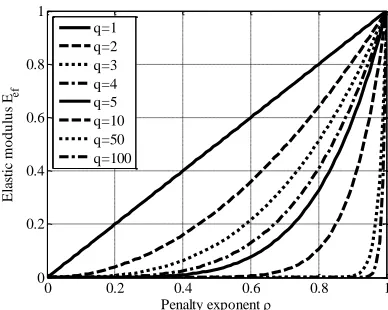
23 Fig. 3 Actual elastic modulus vs. penalty exponent of SIMP method
When SIMP method implemented into FE code, it is based on the assumption that the stiffness matrix of each element is proportional to its density. If E is the actual elastic modulus of the material, Eef = E is defined as the ―effective‖ elastic modulus
of each element, lower than E in design regions with relative pseudo-density lower than 1. The pseudo-density is defined as =q, where is the relative density referred to the actual density of the material and continuously varying between 0 and 1, q is a penalty exponent that, for values sufficiently higher than 1 (normally q>3), makes elements with intermediate values of Eef unfavorable for an economical use of
material, thus highly reducing their number in the optimal solution.
Based on these assumptions, the contribution of elements with nearly 0 to the global stiffness matrix (and therefore to the model compliance), as well as the effect of their removal, is negligible. By referring to the assumed relationship between material properties and density, the design variables were the internal pseudo-densities assigned to each finite element (i), whose stiffness matrix was proportional to E = ρqE.
Discretization with finite elements (numbered as i=1….N) allows to define u and f as the displacement and load vectors, respectively, so that compliance C=fTucould be minimized. The SIMP method was hence performed as a minimum compliance design, where a material distribution problem was to be solved. Since Ku = f, then f
is related to u through the global stiffness matrix K, the latter being proportional to the effective elastic modulus
E
efi=i E of each element i. Hence, if V is the totalvolume of the structure after topology optimization, assigned as a percentage of the actual volume V0 of the structure before the topology optimization process,
minimization of compliance C leads to:
0 0.2 0.4 0.6 0.8 1
0 0.2 0.4 0.6 0.8 1
Penalty exponent
E
la
st
ic
m
o
d
u
lu
s
Eef
24
,
min
ef i i E uf
T
u
(5)and allows to obtain the pseudo-density value i in each element for:
0
i
1
and
0
1
N i i i
V
V
V
(6)After having evaluated the volume V0 before inserting holes, topology optimization
was hence performed by minimizing compliance C (that is maximizing stiffness) for different given VR=(V0V)/V0, thus obtaining a range of solutions.
The SIMP method is a very efficient structural optimization approach that has demonstrated its effectiveness in a large number of examples. It is also the method implemented in many commercial tools (OptiStruct, Genesis, MSC/Nastran, ANSYS, etc.) performing topology optimization. Take the ANSYS for example, the general optimization problem statement of SIMP method implemented in ANSYS is briefly introduced.
The theory of topological optimization seeks to minimize or maximize the objective function (f) subject to the constraints (gj) defined. The design variables (ηi) are
internal pseudo-densities that assigned to each finite element (i) in the topological problem. The pseudo-density for each element varies from 0 to 1, where ηi ≈ 0
represents material to be removed, and ηi ≈ 1 represents material that should be kept.
Stated in simple mathematical terms, the optimization problem is as follows:
f = ηi (min, max) (7)
Subject to:
0
1
1, 2, 3,
,
1, 2, 3,
,
i
j j j
i
n
g
g
g
j
m
(8)CHAPTER 2.STATE-OF-ART:STRUCTURAL OPTIMIZATION
25 Common for all the material interpolation approaches is that they represent smooth, differentiable problems that can efficiently be solved by well-proven, gradient-based optimization approaches such as optimality criteria methods, the method of moving asymptotes (MMA) or by other mathematical programming-based optimization algorithms. Apart from OC methods, these optimizers also immediately allow for systematic and straightforward inclusion of additional global constraints. However, while formally it is easy to include local constraints as well, parameterization issues as seen in stress constrained problems may render such problems quite hard to solve in practise (Sigmund and Maute, 2013).
2.3.2 Evolutionary Structural Optimization (ESO) Method
The evolutionary structural optimization (ESO) technique (Huang and Xie, 2008, Xie and Steven, 1993) was originally proposed in 1992 by Professors Mike Xie and Grant Steven. They aimed to develop a very simple but versatile technique for finding optimal structural designs (Xie and Steven, 1993). ESO is based on the concept of slowly removing inefficient materials from a structure so that the residual structure evolves towards the optimum. Practically all aspects of structural behavior can be accommodated within the ESO concept and the optimality constraints can be stress based, stiffness/displacement based, frequency based, buckling load based, with single or multiple environments.
ESO method uses the concept of gradually removing (―hard-kill‖) redundant material from a structure based on von Mises stress or strain energy of each element so that the resultant structure evolves toward an optimum (Abolbashari and Keshavarzmanesh, 2006). Compared with other existing methods, the ESO method is much more straightforward and involves no mathematical programming techniques in the optimization process. In fact it can be easily implemented into any general purpose finite element analysis (FEA) program (Chu, et al., 1996, Tanskanen, 2002).
26
However, the ESO and BESO may result in a non-optimal when these methods are implemented and used. G. I. N. Rozvany (Rozvany, 2008) gave a critical review of ESO method and pointed out some critics. Such as ESO is fully heuristic and exists no rigorous proof that element eliminations or admissions on the above basis do give an optimal solution, ESO procedure cannot be easily extended to other constraints or to multi-load or multi-constraint problems, it is not particularly efficient if designers have to select the best solution by comparison out of a very large number of intuitively generated solutions. Moreover, he pointed out although ESO usually requires a much greater number of iterations than gradient-type methods, it may yield an entirely non-optimal solution even with respect to ESO’s objective function, and he verified that through a simple example of cantilever beam in a very brief note (Edwards, et al., 2007, Zhou and Rozvany, 2001).
2.3.3 Level Set Method
The level set method (LSM) is a numerical technique proposed by American mathematicians Stanley Osher and James Sethian in the 1980s (Osher and Sethian, 1988) for tracking interfaces and shapes. It has widely application in many disciplines, such as image processing, computer graphics and etc.. In 2000, Sethian and Wiegmann introduced the concept of level set method to structural optimization firstly (Sethian and Wiegmann, 2000, Xia, et al., 2012).
In the level set method, the boundary of the design is defined by the zero level contour of the level set function φ(x) and the structure is defined by the domain where the level set function takes positive values, i.e.
0 :
:
0
1:
:
0
x
x
(9)In the past decade numerous level set methods have emerged which can be classified, for example, by the approach for discretizing the level set function, the approach for mapping the level set field onto the mechanical model, and the approach for updating the level set field in the optimization process (Sigmund and Maute, 2013, Wang, et al., 2003).
CHAPTER 2.STATE-OF-ART:STRUCTURAL OPTIMIZATION
27 remove material in regions of low stress and to add material in regions of high stress. A removal rate is established representing a percentage of the maximal initial stress below which material may be eliminated, and above which material should be added. The biggest benefit of this approach is that it is easier to add material at holes’ boundaries with high stress than on a triangulated finite element mesh. This approach seeks to improve design by making more efficient use of the material (Allaire, et al., 2002, Osher and Fedkiw, 2001, Wang, et al., 2003).
2.3.4 Numerical Instabilities
Although the topology optimization method of continuum structures developed speedily from the landmark paper of Bendsøe and Kikuchi and has reached a level of maturity when applied in structural problems, there still exist a number of problems concerning checkerboard, mesh dependency and local minima.
Checkerboard refers to the problem of formation of regions of alternating solid and void elements ordered in a checkerboard like fashion. The appearance of these regions is due to bad numerical modeling of the stiffness of checkerboards and has nothing to do with the approach no matter of homogenization or SIMP method. Diaz and Sigmund (Diaz and Sigmund, 1995) compared the stiffness of checkerboard configurations in a discretized setting to the stiffness of uniformly distributed materials and concluded that the checkerboard structure has artificially high stiffness, which works provide useful guidelines regarding choice of stable elements (Sigmund and Petersson, 1998).
28
CHAPTER 3. CALATRAVA BRIDGE OF VENICE
29
CHAPTER 3
3. PROPOSED OPTIMIZATION INDEX
Structural optimization has become in the last decades an important mathematical tool for designers. Among the different optimization techniques, sizing and shape optimization allow for identification of structural solutions and layouts characterized by a better exploitation of material, thus decreasing self-weight of structure and saving material costs, topology optimization aids the designers to find the most suitable shape of a structure from a structural and an architectural point of view, which leads to the definition of voids patterns delimiting regions where fluxes of force migrate from force application point to boundary regions.
With the powerful tool of topology optimization, designers can obtain families of candidate solutions by modifying input volume reduction (VR) ratio thus reducing structural weight as much as possible. However, find the best compromise between material saving and structural performance among these candidate solutions is a critical issue for designers. To face this issue, an optimization index (OI) was originally defined concomitantly with the structural optimization of a steel concrete arch bridge built is San Donà in the province of Venice, Italy (Briseghella, et al., 2012). It provides to the designer a mathematical procedure able to highlight the best choice among several candidate solutions obtained by the optimization procedure.
Moreover, during earlier designing phases of a project, in particular in the case of spatial shell structures, several starting trial solutions as well as tentative solutions might being defined based on the judgment of designer, each solution characterized by a particular layout, material property or distribution of boundary conditions. In this case, structural optimization is still a viable tool to optimize structures, but it would led to the definition of entire families of possible candidate solutions, depending on input VR target and tentative starting models through particular layout, different material property or boundary condition. Therefore, the problem is changed from single-family multi-solutions to multi-families multi-solutions.
30
OI*, through the introduction of weight vector w, a further GOI* formulation is presented. The proposed generalized optimization index allows not only to identify best candidate solution originated by a unique reference model, but even comparing structural performances between candidates solution derived by several starting trial solutions.
3.1. Optimum Index Formulation for Single-Family Multi-Solutions
The optimization index (OI) was originally defined by Briseghella et al. 2012, and has been published in the Journal of Bridge Engineering. However, to present to the reader clearly and consecutively, the identified process of OI was introduced in this section again.
During structural optimization, immediately following the topological optimization procedure on structures, several candidate design solutions with voids for each starting layout are generally defined, as many as input volume reductions. Although the design objective of topology optimization is reduction of structure self-weight, the increase of volume reduction generally causes a variation of both stress distribution and deflection level, whose control is therefore a competing requirement with respect to volume reduction itself. Hence, a way of identifying the most suitable design solution that presents the best compromise between material saving and structural performance among all these different optimized layouts with holes has to be defined.
Since a set of optimum layouts with holes were obtained from topology optimization for different values of volume reduction, a specific optimization index was introduced to give the designer a specific mathematical tool to identify the most suitable design solution. Such an index had to take into account volume reduction (and therefore weight reduction) together with the structural response in terms of both stress and deformation level.
CHAPTER 3.CALATRAVA BRIDGE OF VENICE
31 Two Response Indexes (RIs) were then identified in terms of percentage variation of deformation and stress level with respect to their corresponding values obtained in the starting model (without holes) under same loading condition, that is:
0
00 0
, i ; , di d
RI i RI d i
d
(10)
In this index i refers to considered i-th solution,
0 andd
0 are the stress and deformation of starting model (without structural optimization),
i andd
i are the stress and deformation of i-th solution. Response Index (RI) is defined in terms of percentage variation of a parameter representative of the behavior of i-th candidate solution compared to reference one, that is the starting model (without optimization) under the same loading condition.Although the design is focus on the reduction of objective like as superstructure weight, cable volume, reaction force and etc., the increase of volume reduction causes an increase of both stress level and deflections, whose control is therefore a competing requirement with respect to volume reduction.
Hence, a way of identifying the most suitable design solution among all these different optimised layouts with holes had to be defined. For this purpose, the variation of structural response with respect to the variation of volume reduction can be compared by defining the ratio RI/VR as optimization index or, conversely, its complement to 1, that is:
1
1 RI i
OI i VR i RI i
VR i VR i
(11)
VR and RI are the volume reduction and response indexof i-th solution, respectively. Graphical interpretation of optimization index is shown in Fig. 4, in which both VR
and RI are expressed in percent, thus varying between 0 and 100.
Considering the cartesian plane where VR is the x-axis and RI the y-axis, the difference VR-RI represents the distance between the plane bisetrix and the RI
32
axis is VR-(VR-RI)/VR is so obtained (Fig. 4 a). Conversely, a curve whose distance from the bisetrix is VR-(VR-RI)/VR and from the abscissa axis is (VR-RI)/VR can also be obtained (Fig. 4 b). The latter curve is therefore the OI curve defined as above, and therefore expressed in percent as VR and RI.
Fig. 4 Graphical interpretation of optimization index
Since the optimization objective was lightening the bridge in most specific engineering case, it was then worth modifying the scaling coefficient 1/VR through a penalty exponent able to favour design solutions with higher volume reduction. For this purpose, after introduction of the penalty exponent, the scaling coefficient became (1/VR), where values of the penalty exponent between 0 and 1 favour design solutions with higher volume reduction, while values higher than 1 favour design solutions with higher performances but higher self-weight, and therefore not convenient to lighten the bridge (Fig. 4 c). Hence, the updated expression of the optimization index OI through introduction of the penalty exponent is:
1
OI i VR i RI i
VR i
(12)
is a penalty exponent, usually between 0 and 3, able to favor design solutions with lower or higher volume reduction according to is higher of lower than 1. The application of the penalty exponent to the scaling factor 1/VR results therefore in lower values of OI for <1 and in higher values for >1.
CHAPTER 3.CALATRAVA BRIDGE OF VENICE
33 the scaling factor (1/VR) plotted as a function of VR approaches a hyperbole for closer to tending to become an horizontal line for closer to
Hence, while for >1 design layouts with holes are not favoured and those with low values of volume reduction are conversely favoured already for slightly higher than 1, for <1 design solutions with high volume reduction are instead favoured, the higher the volume reduction the lower is .
Fig. 5 Scaling factor 1/VR with penalty exponent vs. VR
In the right chart of Fig. 5, the ratio R((1/VR)/(1/VR) is plotted for different values of . It can be seen that for 2the ratio R(2) is roughly 0 for almost every value of
VR. On the contrary, for 0.5 the ratio R(0.5) is a steep function of VR, meaning that the scaling factor with penalty exponent 0.5 becomes much higher than the one without the penalty exponent evenfor low values of VR, becoming 10 times 1/VR for
VR=100%. An intermediate trend is observed for 8, with R initially slightly steep, and then even less steep until the value of only 2.5 times 1/VR is reached for
VR=100%.
Hence, although in general values of less than 1 favour design solutions with significant volume reduction, values of less than but suitably close to 1 are able to favour design solutions with intermediate values of volume reduction.
Eventually, since the expression of the above optimization index is referred to a specific structural response in terms of stress or deformation, a global optimization index (GOI) considering both these features of structural response can be also defined. By giving the same weight to both deformation and stress level, a global optimization index averaging the two optimization indexes referred to stresses and deformations is then defined as:
0 20 40 60 80 100
0 0.1 0.2 0.3 0.4 0.5
VR(%)
1