Optimizing Back-Propagation Gradient for Classification by an Artificial Neural Network

(1)

Published online August 10, 2014 (http://www.sciencepublishinggroup.com/j/ajpa) doi: 10.11648/j.ajpa.20140204.11

ISSN: 2330-4286 (Print); ISSN:2330-4308 (Online)

Optimizing back-propagation gradient for classification

by an artificial neural network

Said El Yamani, Samir Zeriouh, Mustapha Boutahri, Ahmed Roukhe

Optronic and Information Treatment Team, Atomic, Mechanical, Photonic and Energy Laboratory, Faculty of Science, Moulay Ismail University, B. P. 11201 Zitoune, Meknès, Morocco

Email address:

[email protected] (S. E. Yamani)

To cite this article:

Said El Yamani, Samir Zeriouh, Mustapha Boutahri, Ahmed Roukhe. Optimizing Back-Propagation Gradient for Classification by an Artificial Neural Network. American Journal of Physics and Applications. Vol. 2, No. 4, 2014, pp. 88-94.

doi: 10.11648/j.ajpa.20140204.11

Abstract:

In a complex and changing a remote sensing system, which requires taking quick and informed decisions environment, connectionist methods have shown their great contribution in particular the reduction and classification of spectral data. In this context, this paper proposes to study the parameters that optimize the results of an artificial neural network ANN multilayer perceptron based, for classification of chemical agents on multi-spectral images. The mean squared error cost function remains one of the major parameters of the network convergence at its learning phase and a challenge that will face our approach to improve the gradient descent by the conjugate gradient method that seems fast and efficient.

Keywords: Optimizing, Artificial Neural Networks, Classification, Identification, Conjugate Gradient,

Multi-Layer Perceptron, Back Propagation of the Gradient

1. Introduction

Recent years have been marked by an extraordinary emergence of Artificial Neural Networks (ANNs) that were found very suitable for solving complex and unstructured classifications. The strength of these actually lies in their ability to adapt thanks to a learning phase through which they develop and establish relationships between variable from a dataset. In the field of remote sensing, ANN proved of great interest among researchers especially in case of non-linear phenomena.

Nowadays, several threats proliferate and the most important remain chemical, biological or nuclear. These threats can occur in several scenarios and require immediate action. It should be noted that, facing such an eventuality, a large number of key elements turns essentially necessary to determine the particular nature or agents, their rates, their propagation speeds and especially the surfaces they could occupy.

This involves the deployment of resources and identification of reliable and efficient classification. In this context the ANN appear to be a highly suitable tool [1].

Their diverse neuronal architectures allow justifying the choice of the type of neural networks to use for each case

that may arise. In addition, during emergency cases, many optimization methods are proposed to reduce processing time and improve network performance, considering these constraints and characteristics related to the use of the type of network selected.

Thus, the work of this paper focuses on this subject to the optimization of the back propagation learning in the network.

2. Multi-Layer Perceptron Network

2.1. MLP Network Architecture

The model used is a Multi-layer Perception based (MLP) network, comprising a P layer of n inputs, the hidden layers and a Y layer of m outputs [2]. Adjacent layers are fully connected (Fig. 1).

(2)

The number of cells in each hidden layer may vary depending on the behavior of the network. However, the number of cells of the output layer corresponds to the dimension of projection which is 3.

Activation functions adopted in this ANN model are sigmoid and linear for the output function.

Diagram 1 shows a simplified diagram of the network.

2.2. Learning Algorithm

2.2.1. Back Propagation of Gradient

The proposed algorithm is the back propagation gradient that helps learning the multi-layer network characteristics by updating and adjusting the weights of different layers to minimize a cost function [3].

Figure 1. MLP network architecture.

Diag 1. Simplified model of MLP network architecture.

Where bjis the total input of the output layer sk and ak is

the total input of the hidden layer yj.

It goes through three phases: A first one that allows forward propagation of the cells state. The second step is a back propagation process that minimizes the error, and the third step is an adjustment of the weights connection [4].

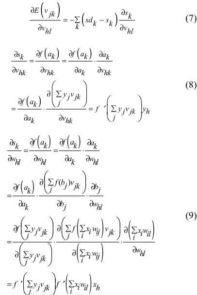
Mathematical expressions of the different phases of the algorithm are expressed by the following equations.

First, the cost function “E” must be defined:

( )

(

)

2

1 2

E v_jk s_d s_k k k

∑

= − (3)

Where, Sdk is the desired output; Sk is the effective

To minimize E, we calculate its gradient with respect to the weightsν, then we change the weight in the opposite direction of the gradient. In other words, we update the weights of the gradient of the highest slope.

( )

1

E v jk v jk

v jk

η ∂

∆ = −

∂ (4)

1

n n n

jk jk jk

v

=

v

+

− ∆

v

(5) Where, η (0< η <1) is the gradient step, used to control the fast convergence of the algorithm.

For a two-layer network:

( )

s_k f y v_j _jk f f x w_{i ij} v_jk

j j i

∑ ∑ ∑

=  =  

    (6)

After partial derivations, respectively to vhl and whl, we

obtain:

( )

₍

₎

E v_jk _s

k sd_k s_k k

v_hl v_hl

∂ _∂

∑

= − −

∂ ∂ (7)

( )

f a f a

s_k _k _k a_k

v_hk v_hk a_k v_hk

y v_{j jk} f a_k j

f y v_{j jk} y_h j

a_k v_hk

∂ ∂ ∂ ∂ = = ⋅ ∂ ∂ ∂ ∂ ∑ ∂ ∂ ∑ = ⋅ = ′ ∂ ∂     _ _       (8)

( ) ( )

( )

f a f a s_k _k _k a_k

w_hl w_hl a_k w_hl

f b v_{j jk} b

f a_k _j _j

a_k b_j w_hl

f _jy vj jk _jf _ix w vi ij jk x w_{i il} i

w

x w hl

y v_{j jk} _i i ij j

f y v_j _jk f x w_i _il x_h

j i ∂ ∂ ∂ ∂ = = ⋅ ∂ ∂ ∂ ∂ ∑ ∂ _∂ ∂ = ⋅ ⋅ ∂ ∂ ∂ ∑ ∑ ∑ ∂ ∂ ∂∑ = ⋅ ⋅ ∂ ∑ ∂ ∑ ∂ ∑ ∑ = ′ ′















 





 





 



























(9)

Substituting the derivatives in the weights updating equations, we get:

(

)

1

v_hl sd_l s_l f y w_j _jl y_h j

l

η ∑ ∑

∆ = − ′ 

  (10)

( )

2

w_hl f y w_j _jl f x w_i _il x_h

j i

η ∑ ∑

∆ = ′  ′

  (11)

2.2.2. Back Propagation of Gradient (Method of Newton)

(3)

( ) ( )

( )

( ) ( )

1 2 1 2 n E v_jk

n n n

E v_jk E v_jk _m v_jk m _v

n E v

T _jk

n n

v_jk _m _p v_jk m p _v _v

∂ + ₌ ₊_∑ _{⋅ ∆} ∂ ∂ ∑ ∑ + ∆ ⋅ ∆ ∂ ∂









(12)

Where

∆

( )

v

n_jk

=

v

n_jk+1

−

v

n_jk To simplify,

( ) ( ) ( ) ( )

( )

( ) ( )

1 1 2

n n n n

E v_jk E v_jk E v_jk v_jk

T

n n n

v_jk E v_jk v_jk

+ ₌ ₊ ′ _{⋅ ∆}

′′ +



_

∆



_

⋅ ∆

(13)

Where the E’ matrix composed of partial derivatives of 1st order is a jacobian matrix:

( ) ( )

E v jkn

n n

G _{E vjk}

m m _{v jk}

∂

′ _∑

= =

∂

(14)

And E’’ is a matrix composed of second order partial derivatives, which is a Hessian symmetric positive definite matrix:

( )

2E vjk

( )

n

n n

H E _{v jk}

p m m p v_jk v_jk

∂

′′ _∑∑

= =

∂ ∂

(15)

Deriving from (13)

( ) ( ) ( ) ( )

n1 n n n

E v′ _jk+ =E v′ _jk +E′′ v_jk ∆ v_jk (16)

We assume E' and E'' are continuous and exist for values of higher order derivatives, very negligible for this approximation to be minimized.

From (16), the weights updating can be expressed as:

( ) ( ) ( )

1

n n n

v_jk E v_jk E v_jk

−

′ ′′

∆ = − ⋅



_



_

(17)

( ) ( )

1

n n n n

v_jk v_jk E v_jk E v_jk

− + ₌ ₋



′

 

_⋅ ′′





 



(18)

1 1

n n n m

jk jk

v

+

= −

v

  

_{  }

G

⋅

H



_

− (19) From (17), the gradient can be expressed as:

(

1

)

n n n n

G = −H ⋅ v+ −v (20)

To improve this method, we try to make Gn+1 orthogonal to the line of the previous value of Gn. So, we pose:

( )

1 0

T

n n

G+ G = (21)

After weight adjustments according to (5)

1

n n n n

v+ − = −v η G (22)

And after substitution of (16)

1

n n n n n

G+ = −G η H G (23)

Finally, multiplying this result by (Gn)T leads to:

( )

0

T T

n n n n n n G G η G H G

= − (24)

Hence, from this last one, we obtain

( )

T n n G G n T n n n G H G

η = (25)

Note that Hn are constant:

For n=0 G1=G0+H0⋅

( )

v1−v0 (26)

Where the minimal error is obtained for G1=0. That means:

( )

1

1 0 0 0

v v H G

−

− = − (27)

This corresponds to the results of the Newton's method, which is for updating weights:

( )

1

0

n n n

v v G H

n

−

∑

− = − (28)

Thus, the weights are updated in the direction of negative gradient following form:

0

n n n

v

− =−

v

α

G

(29) However the major disadvantage of this method is the calculation of the storage and the inversion of the Hessian matrix during iterations. This is why the conjugate gradient method, a quasi-Newton method likely to reduce these limitations, reveals more efficient.

2.2.3. Methods of Improving Back-Propagation Gradient 2.2.3.1. Method of BGFS (Quasi-Newton)

This algorithm is the Broyden-Fletcher-Goldfarb- Shanno. The weight update is made according to the equation [6]:

( )

T

n n n

v H G

(4)

2.2.3.2. Method of Levenberg-Marquardt (LM)

This is a similar method to the BFGS algorithm with

( )

_n T

( ) ( )

T

H = ∇E ⋅ ∇E et G= ∇

( )

G T⋅ε where ∇G is the

jacobian matrix of 1st order, and ε is the errors vector [7].

2.2.3.3. Method of Gradient Descent with Momentum

To prevent learning phases causes oscillations, the weight difference comprises varying the previous weight by adding a kinetic energy term [8].

1

n n n n

v

α

G

ρ

v

−

∆ =−

+ ∆

(31)

2.2.3.4. Method of the Conjugate Gradient

The conjugate gradient method is similar to the descent of the steepest approach, but includes an inertial term which is calculated during iterations steps to search for the conjugate of the directions, the update process has been described by Fletcher -Reeves of the Polak-Ribiere [9].

According to Fletcher-Reeves, we operate on it, firstly by looking for the most important downward slope, and then by combining its direction with the previous one.

0 0

G g

− = , ∆vn_jk= −αn ng

1

n n n n

g = −G +β g − ,

( )

1 1

T

n n

G G

n

T

n n

G G

β = +

− ₊ − (32)

Or

( )

1

1 1

T

n n

G G

n

T

n n

G G

β

−

∆ +

=

− ₊ − Polak-Ribiere according

3. Application in Chemicals Agents

Identification and Classification

3.1. Classification Using Multi-Layer Perceptron

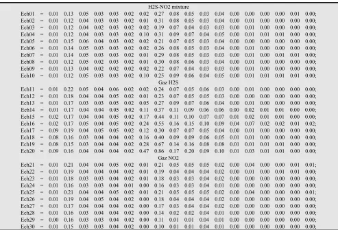
In order to implement the followed theoretical process, a program has been written using Matlab and applies for a database with sample of the three agents (Table 1).

Table 1. Three agents gas database.

H2S-NO2 mixture

Ech01 = 0.01 0.13 0.05 0.03 0.03 0.02 0.02 0.27 0.08 0.05 0.03 0.04 0.00 0.00 0.00 0.00 0.01 0.00; Ech02 = 0.01 0.12 0.04 0.03 0.03 0.02 0.01 0.31 0.08 0.05 0.03 0.04 0.00 0.01 0.00 0.00 0.00 0.00; Ech03 = 0.01 0.12 0.04 0.02 0.03 0.02 0.02 0.19 0.07 0.04 0.03 0.03 0.00 0.01 0.00 0.00 0.00 0.00; Ech04 = 0.01 0.12 0.04 0.03 0.03 0.02 0.10 0.31 0.09 0.07 0.04 0.05 0.00 0.01 0.01 0.01 0.00 0.00; Ech05 = 0.01 0.15 0.06 0.04 0.03 0.02 0.02 0.21 0.07 0.05 0.03 0.04 0.00 0.00 0.00 0.00 0.00 0.00; Ech06 = 0.01 0.14 0.05 0.03 0.03 0.02 0.02 0.26 0.08 0.05 0.03 0.04 0.00 0.01 0.00 0.00 0.00 0.00; Ech07 = 0.01 0.14 0.05 0.03 0.03 0.02 0.01 0.29 0.08 0.05 0.03 0.03 0.00 0.01 0.00 0.01 0.01 0.00; Ech08 = 0.01 0.12 0.05 0.02 0.03 0.02 0.01 0.30 0.08 0.06 0.03 0.04 0.00 0.01 0.00 0.00 0.00 0.00; Ech09 = 0.01 0.13 0.04 0.02 0.02 0.02 0.02 0.22 0.07 0.04 0.03 0.03 0.00 0.01 0.00 0.00 0.00 0.00; Ech10 = 0.01 0.12 0.05 0.03 0.03 0.02 0.10 0.25 0.09 0.06 0.04 0.05 0.00 0.01 0.01 0.01 0.01 0.00;

Gaz H2S

Gaz NO2

The followed methodology during this computing phase in Matlab is based on fundamental steps, especially the creation of the network where

The Samples matrix that contains the input values of the network are r × s = 18 × 30 size;

The matrix with the desired results. Its size is 3× 30 with the following vectors [-1 -1 +1]’, [-1 +1 -1]’ and [+1 -1 -1]’ as expected result per type of gas.

(5)

The outputs of the networks at each iteration are equivalent to the expected values in the samples where the total learning path length is associated to a gradient and E (Fig. 5).

The initial weights have values near zero.

3.2. Matlab Simulations

We conducted various simulations in Matlab for testing and the results are plotted as follow:

Figure 2. 3D classification of the three agents and performances in learning with Gradient Descent (GD) (traingd)

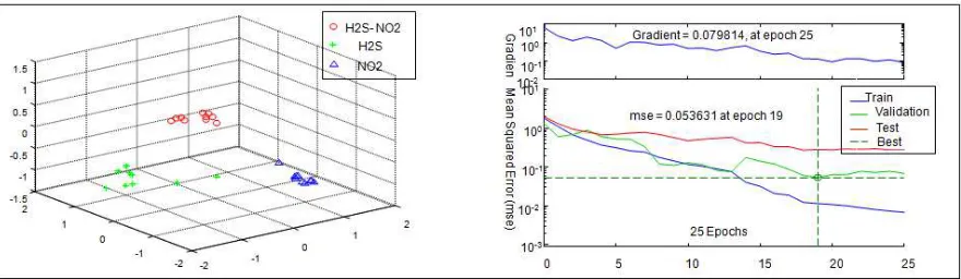
Figure 3. 3D classification of the three agents and performances in learning with Levenberg-Marquardt (LM) (trainlm)

Figure 4. 3D classification of the three agents and performances in learning with GD with Momentum (GDM) (traingdm)

(6)

Figure 6. 3D classification of the three agents and performances in learning with CGD Fletcher-Reeves (traincgf)

Figure 7. 3D classification of the three agents and performances in learning with CGD Polak-Ribière (traincgp)

Figure 8. 3D classification of the three agents and performances in learning with Quasi-Newton (BFGS) (trainbfg)

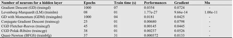
Table 2. Comparison of parameters of the different back-propagation networks

Number of neurons for a hidden layer Epochs Train time (s) Performances Gradient Mu

Gradient Descent (GD) (traingd) 1000 07 0.0354 0.0724 - Levenberg-Marquardt (LM) (trainlm) 08 01 1.77e-27 9.66e-14 1.00e-11 GD with Momentum (GDM) (traingdm) 1000 04 0.0181 0.0425 - Conjugate Gradient Descent (trainscg) 25 01 0.00680 0.0798 - CGD Fletcher-Reeves (traincgf) 45 01 0.00145 0.0445 -

CGD Polak-Ribière (traincgp) 38 01 0.00237 0.0526 -

Quasi-Newton (BFGS) (trainbfg) 37 31 0.000372 0.0133 -

3.3. Results Analysis

The simulation results obtained show that, the back-propagation of the gradient, which operates an iterative approximation along the line of the steepest slope, could be improved by the conjugate gradient algorithm with the search for a minimum which produces a faster convergence, and could also be improved by the Quasi-Newton method. However, in this case, this remains less efficient than the Levenberg-Marquardt. Compared to other back-propagation

algorithms, the latter is much more effective in view of its high speed and high precision, considering the network does not reach saturation.

4. Conclusions

(7)

classification of chemical agents. This classification is applied to a database which test statistic is the mean square error to be minimized to threshold value. From this study, it appears that multiple solutions are able to optimize the performance of learning, thereby creating special interest in functional classification.

So if back propagation algorithms adjust the weights in the direction of greatest slope, direction in which the performance function decreases more rapidly, it is still possible that convergence can be made faster with the conjugate gradient algorithm or the Quasi-Newton method for fast optimization algorithm or Levenberg-Marquardt. The latter was designed for second order training approaches without having to calculate the Hessian matrix. Thanks to the implementation done in MATLAB, this algorithm seems to be very effective in classification problems of moderate size of this kind, in spite of its very high calculations at iterations.

References

[1] M. JANATI IDRISS and All, Reducing the number of channels of multi-spectral images by connectionist approach, Signal Processing 17, 2000, pp 491-500.

[2] A. Guerin, J.H. Crasy, Reconfigurable computing architecture for simulating networks of neurons, Review Signal Processing 5 (3), 1988, pp 178-186.

[3] J. Proriol, MLP: Network program multi-layer neurons, Journal of Modulad, 1996, pp 24-28.

[4] S. Lahmiri, A comparative study of back-propagation algorithms in financial prediction, International Journal of Computer Science, Engineering and Applications (IJCSEA), Vol.1, No.4, 2011, pp 15-21.

[5] L. N. M. Tawfiq Improving Gradient Descent Method for Training Feed Forward Neural Networks, International Journal of Modern Computer Science & Engineering, 2(1), 2013, pp 12-24.

[6] M. F. MEILLER, A Scaled Conjugate Gradient Algorithm for Fast Supervised Learning, Neural Networks, Vol.6, 1993, pp. 525-533.

[7] M. Wilamowski, and Hao Yu Improved Computation for Levenberg–Marquardt Training, IEEE transactions on neural networks, vol. 21, no. 6, 2010, pp 930-93.

[8] N. Qian1, On the momentum term in gradient descent learning algorithms, Neural Networks, 1999, pp 145-151. [9] R. S. Ransing and N. M. Nawi1, An improved conjugate

gradient based learning algorithm for back propagation neural networks, World Academy of Science, Engineering and Technology, Vol 2, 2008, pp 06-26.