Randomized Variable Elimination
David J. Stracuzzi [email protected]
Paul E. Utgoff [email protected]
Department of Computer Science University of Massachusetts at Amherst 140 Governors Drive
Amherst, MA 01003, USA
Editor: Haym Hirsh
Abstract
Variable selection, the process of identifying input variables that are relevant to a particular learning problem, has received much attention in the learning community. Methods that employ a learning algorithm as a part of the selection process (wrappers) have been shown to outperform methods that select variables independently from the learning algorithm (filters), but only at great compu-tational expense. We present a randomized wrapper algorithm whose compucompu-tational requirements are within a constant factor of simply learning in the presence of all input variables, provided that the number of relevant variables is small and known in advance. We then show how to remove the latter assumption, and demonstrate performance on several problems.
1. Introduction
When learning in a supervised environment, a learning algorithm is typically presented with a set of N-dimensional data points, each with its associated target output. The learning algorithm then outputs a hypothesis describing the function underlying the data. In practice, the set of N input variables is carefully selected by hand in order to improve the performance of the learning algorithm in terms of both learning speed and hypothesis accuracy.
In some cases there may be a large number of inputs available to the learning algorithm, few of which are relevant to the target function, with no opportunity for human intervention. For example, feature detectors may generate a large number of features in a pattern recognition task. A second possibility is that the learning algorithm itself may generate a large number of new concepts (or functions) in terms of existing concepts. Valiant (1984), Fahlman and Lebiere (1990), and Kivinen and Warmuth (1997) all discuss situations in which a potentially large number of features are created during the learning process. In these situations, an automatic approach to variable selection is required.
In spite of the cost, variable selection can play an important role in learning. Irrelevant variables can often degrade the performance of a learning algorithm, particularly when data are limited. The main computational cost associated with the wrapper method is usually that of executing the learn-ing algorithm. The learner must produce a hypothesis for each subset of the input variables. Even greedy selection methods (Caruana and Freitag, 1994) that ignore large areas of the search space can produce a large number of candidate variable sets in the presence of many irrelevant variables.
Randomized variable elimination avoids the cost of evaluating many variable sets by taking large steps through the space of possible input sets. The number of variables eliminated in a single step depends on the number of currently selected variables. We present a cost function whose pur-pose is to strike a balance between the probability of failing to select successfully a set of irrelevant variables and the cost of running the learning algorithm many times. We use a form of backward elimination approach to simplify the detection of relevant variables. Removal of any relevant vari-able should immediately cause the learner’s performance to degrade. Backward elimination also simplifies the selection process when irrelevant variables are much more common than relevant variables, as we assume here.
Analysis of our cost function shows that the cost of removing all irrelevant variables is dom-inated by the cost of simply learning with all N variables. The total cost is therefore within a constant factor of the cost of simply learning the target function based on all N input variables, provided that the cost of learning grows at least polynomially in N. The bound on the complexity of our algorithm is based on the complexity of the learning algorithm being used. If the given learn-ing algorithm executes in time O(N2), then removing the N−r irrelevant variables via randomized variable elimination also executes in time O(N2). This is a substantial improvement compared to the factor N or more increase experienced in removing inputs one at a time.
2. Variable Selection
The specific problem of variable selection is the following: Given a large set of input variables and a target concept or function, produce a subset of the original input variables that predict best the target concept or function when combined into a hypothesis by a learning algorithm. The term “predict best” may be defined in a variety of ways, depending on the specific application and selection algorithm. Ideally the produced subset should be as small as possible to reduce training costs and help prevent overfitting.
From a theoretical viewpoint, variable selection should not be necessary. For example, the pre-dictive power of Bayes rule increases monotonically with the number of variables. More variables should always result in more discriminating power, and removing variables should only hurt. How-ever, optimal applications of Bayes rule are intractable for all but the smallest problems. Many machine learning algorithms perform sub-optimal operations and do not conform to the strict con-ditions of Bayes rule, resulting in the potential for a performance decline in the face of unnecessary inputs. More importantly, learning algorithms usually have access to a limited number of exam-ples. Unrelated inputs require additional capacity in the learner, but do not bring new information in exchange. Variable selection is thus a necessary aspect of inductive learning.
networks, known as parameter pruning. These methods cannot directly perform variable selection for arbitrary learning algorithms; they are approaches to removing irrelevant inputs from learning elements.
Many variable selection algorithms (although not all) perform some form of search in the space of variable subsets as part of their operation. A forward selection algorithm begins with the empty set and searches for variables to add. A backward elimination algorithm begins with the set of all variables and searches for variables to remove. Optionally, forward algorithms may occasionally choose to remove variables, and backward algorithms may choose to add variables. This allows the search to recover from previous poor selections. The advantage of forward selection is that, in the presence of many irrelevant variables, the size of the subsets will remain relatively small, helping to speed evaluation. The advantage of backward elimination is that recognizing irrelevant variables is easier. Removing a relevant variable from an otherwise complete set should cause a decline in the evaluation, while adding a relevant variable to an incomplete set may have little immediate impact.
2.1 Filters
Filter methods use statistical measures to evaluate the quality of the variable subsets. The goal is to find a set of variables that is best with respect to the specific quality measure. Determining which variables to include may either be done via an explicit search in the space of variable subsets, or by numerically weighting the variables individually and then selecting those with the largest weight. Filter methods often have the advantage of speed. The statistical measures used to evaluate variables typically require very little computation compared to cost of running a learning algorithm many times. The disadvantage is that variables are evaluated independently, not in the context of the learning problem.
Early filtering algorithms include FOCUS (Almuallim and Dietterich, 1991) and Relief (Kira and Rendell, 1992). FOCUS searches for a smallest set of variables that can completely discriminate between target classes, while Relief ranks variables according to a distance metric. Relief selects training instances at random when computing distance values. Note that this is not related to our approach of selecting variables at random.
Decision trees have also been employed to select input variables by first inducing a tree, and then selecting only those variables tested by decision nodes (Cardie, 1993; Kubat et al., 1993). In another vein, Koller and Sahami (1996) discuss a variable selection algorithm based on cross entropy and information theory.
Methods from statistics also provide a basis for a variety of variable filtering algorithms. Correlation-based feature selection (CFS) (Hall, 1999) attempts to find a set of variables that are each highly correlated with the target function, but not with each other. The ChiMerge (Kerber, 1992) and Chi2 algorithms (Liu and Setiono, 1997) remove both irrelevant and redundant variables using aχ2test to merge adjacent intervals of ordinal variables.
Discussion of filtering methods for variable selection also arises in the pattern recognition liter-ature. For example, Devijver and Kittler (1982) discuss the use of a variety of linear and non-linear distance measures and separability measures such as entropy. They also discuss several search al-gorithms, such as branch and bound and plus l-take away r. Branch and bound is an optimal search technique that relies on a careful ordering of the search space to avoid an exhaustive search. Plus l-take away r is more akin to the standard forward and backward search. At each step, l new variables are selected for inclusion in the current set and r existing variables are removed.
2.2 Wrappers
Wrapper methods attempt to tailor the selection of variables to the strengths and weaknesses of specific learning algorithms by using the performance of the learner to evaluate subset quality. Each candidate variable set is evaluated by executing the learning algorithm given the selected variables and then testing the accuracy of the resulting hypotheses. This approach has the advantage of using the actual hypothesis accuracy as a measure of subset quality. The problem is that the cost of repeatedly executing the learning algorithm can quickly become prohibitive. Nevertheless, wrapper methods do tend to outperform filter methods. This is not surprising given that wrappers evaluate variables in the context of the learning problem, rather than independently.
2.2.1 ALGORITHMS
John, Kohavi, and Pfleger (1994) appear to have coined the term “wrapper” while researching the method in conjunction with a greedy search algorithm, although the technique has a longer history (Devijver and Kittler, 1982). Caruana and Freitag (1994) also experimented with greedy search methods for variable selection. They found that allowing the search to either add variables or remove them at each step of the search improved over simple forward and backward searches. Aha and Bankert (1994) use a backward elimination beam search in conjunction with the IB1 learner, but found no evidence to prefer this approach to forward selection. OBLIVION (Langley and Sage, 1994) selects variables for the nearest neighbor learning algorithm. The algorithm uses a backward elimination approach with a greedy search, terminating when the nearest neighbor accuracy begins to decline.
Subsequent work by Kohavi and John (1997) used forward and backward best-first search in the space of variable subsets. Search operators generally include adding or removing a single variable from the current set. This approach is capable of producing a minimal set of input variables, but the cost grows exponentially in the face of many irrelevant variables. Compound operators generate nodes deep in the search tree early in the search by combining the best children of a given node. However, the cost of running the best-first search ultimately remains prohibitive in the presence of many irrelevant variables.
Hoeffding races (Maron and Moore, 1994) take a different approach. All possible models (se-lections) are evaluated via leave-one-out cross validation. For each of the N evaluations, an error confidence interval is established for each model. Models whose error lower bound falls below the upper bound of the best model are discarded. The result is a set of models whose error is insignifi-cantly different.
Genetic algorithms have been also been applied as a search mechanism for variable selection. Vafaie and De Jong (1995) describe using a genetic algorithm to perform variable selection. They used a straightforward representation in which individual chromosomes were bit-strings with each bit marking the presence or absence of a specific variable. Individuals were evaluated by training and then testing the learning algorithm. In a similar vein, SET-Gen (Cherkauer and Shavlik, 1996) used a fitness (evaluation) function that included both the accuracy of the induced model and the comprehensibility of the model. The learning model used in their experiments was a decision tree and comprehensibility was defined as a combination of tree size and number of features used. The FSS-EBNA algorithm (Inza et al., 2000) used Bayesian Networks to mate individuals in a GA-based approach to variable selection.
The relevance-in-context (RC) algorithm (Domingos, 1997) is based on the idea that some fea-tures may only be relevant in particular areas of the instance space for instance based (lazy) learners. Clusters of training examples are formed by finding examples of the same class with nearly equiva-lent feature vectors. The features along which the examples differ are removed and the accuracy of the entire model is determined. If the accuracy declined, the features are restored and the failed ex-amples are removed from consideration. The algorithm continues until there are no more exex-amples to consider. Results showed that RC outperformed other wrapper methods with respect to a 1-NN learner.
2.2.2 LEARNER SELECTIONS
Many learning algorithms already contain some (possibly indirect) form of variable selection, such as pruning in decision trees. This raises the question of whether the variable selections made by the learner should be used by the wrapper. Such an approach would almost certainly run faster than methods that rely only on the wrapper to make variable selections. The wrapper selects variables for the learner, and then executes the learner. If the resulting hypothesis is an improvement, then the wrapper further removes all variables not used in the hypothesis before continuing on with the next round of selections.
This approach assumes the learner is capable of making beneficial variable selections. If this were true, then both filter and wrapper methods would be largely irrelevant. Even the most so-phisticated learning algorithms may perform poorly in the presence of highly correlated, redundant or irrelevant variables. For example, John, Kohavi, and Pfleger (1994) and Kohavi (1995) both demonstrate how C4.5 (Quinlan, 1993) can be tricked into making bad decisions at the root. Vari-ables highly correlated with the target value, yet ultimately useless in terms of making beneficial data partitions, are selected near the root, leading to unnecessarily large trees. Moreover, these bad decisions cannot be corrected by pruning. Only variable selection performed outside the context of the learning algorithm can recognize these types of correlated, irrelevant variables.
2.2.3 ESTIMATINGPERFORMANCE
is an expensive procedure, requiring the learner to produce several hypotheses for each selection of variables.
2.3 Model Specific Methods
Many learning algorithms have built-in variable (or parameter) selection algorithms which are used to improve generalization. As noted above, decision tree pruning is one example of built-in variable selection. Connectionist algorithms provide several other examples, known as parameter pruning. As in the more general variable selection problem, extra weights (parameters) in a network can degrade the performance of the network on unseen test instances, and increase the cost of evaluat-ing the learned model. Parameter prunevaluat-ing algorithms often suffer the same disadvantages as tree pruning. Poor choices made early in the learning process can not usually be undone.
One method for dealing with unnecessary network parameters is weight decay (Werbos, 1988). Weights are constantly pushed toward zero by a small multiplicitive factor in the update rule. Only the parameters relevant to the problem receive sufficiently large weight updates to remain signifi-cant. Methods for parameter pruning include the optimal brain damage (OBD) (LeCun et al., 1990) and optimal brain surgeon (OBS) (Hassibi and Stork, 1993) algorithms. Both rely on the second derivative to determine the importance of connection weights. Sensitivity-based pruning (Moody and Utans, 1995) evaluates the effect of removing a network input by replacing the input by its mean over all training points. The autoprune algorithm (Finnoff et al., 1993) defines an importance metric for weights based on the assumption that irrelevant weights will become zero. Weights with a low metric value are considered unimportant and are removed from the network.
There are also connectionist approaches that specialize in learning quickly in the presence ir-relevant inputs, without actually removing them. The WINNOW algorithm (Littlestone, 1988) for Boolean functions and the exponentiated gradient algorithm (Kivinen and Warmuth, 1997) for real-valued functions are capable of learning linearly separable functions efficiently in the presence of many irrelevant variables. Exponentiated gradient algorithms, of which WINNOW is a special case, are similar to gradient descent algorithms, except that the updates are multiplicative rather than ad-ditive.
The result is a mistake bound that is linear in the number of relevant inputs, but only logarithmic in the number of irrelevant inputs. Kivinen and Warmuth also observed that the number of examples required to learn an accurate hypothesis also appears to obey these bounds. In other words, the num-ber of training examples required by exponentiated gradient algorithms grows only logarithmicly in the number of irrelevant inputs.
Exponentiated gradient algorithms may be applied to the problem of separating the set of rel-evant variables from irrelrel-evant variables by running them on the available data and examining the resulting weights. Although exponentiated gradient algorithms produce a minimum error fit of the data in non-separable problems, there is no guarantee that such a fit will rely on the variables rele-vant to a non-linear fit.
3. Setting
Our algorithm for randomized variable elimination (RVE) requires a set (or sequence) of N-dimensional vectors xi with labels yi. The learning algorithm
L
is asked to produce a hypothesis h based onlyon the inputs xi j that have not been marked as irrelevant (alternatively, a preprocessor could remove
variables marked irrelevant). We assume that the hypotheses bear some relation to the data and input values. A degenerate learner (such as one that produces the same hypothesis regardless of data or input variables) will in practice cause the selection algorithm ultimately to select zero vari-ables. This is true of most wrapper methods. For the purposes of this article, we use generalization accuracy as the performance criteria, but this is not a requirement of the algorithm.
We make the assumption that the number r of relevant variables is at least two to avoid degen-erate cases in our analysis. The number of relevant variables should be small compared to the total number of variables N. This condition is not critical to the functionality of the RVE algorithm; how-ever the benefit of using RVE increases as the ratio of N to r increases. Importantly, we assume that the number of relevant variables is known in advance, although which variables are relevant remains hidden. Knowledge of r is a very strong assumption in practice, as such information is not typically available. We remove this assumption in Section 6, and present an algorithm for estimating r while removing variables.
4. The Cost Function
Randomized variable elimination is a wrapper method motivated by the idea that, in the presence of many irrelevant variables, the probability of successfully selecting several irrelevant variables simultaneously at random from the set of all variables is high. The algorithm computes the cost of attempting to remove k input variables out of n remaining variables given that r are relevant. A sequence of values for k is then found by minimizing the aggregate cost of removing all N−r irrelevant variables. Note that n represents the number of remaining variables, while N denotes the total number of variables in the original problem.
The first step in applying the RVE algorithm is to define the cost metric for the given learning algorithm. The cost function can be based on a variety of metrics, depending on which learning algorithm is used and the constraints of the application. Ideally, a metric would indicate the amount of computational effort required for the learning algorithm to produce a hypothesis.
For example, an appropriate metric for the perceptron algorithm (Rosenblatt, 1958) might relate to the number of weight updates that must be performed, while the number of calls to the data purity criterion (e.g. information gain (Quinlan, 1986)) may be a good metric for decision tree induction algorithms. Sample complexity represents a metric that can be applied to almost any algorithm, allowing the cost function to compute the number of instances the learner must see in order to remove the irrelevant variables from the problem. We do not assume a specific metric for the definition and analysis of the cost function.
4.1 Definition
The first step of defining the cost function is to consider the probability
p+(n,r,k) = k−1
∏
i=0
n−r−i n−i
of successfully selecting k irrelevant variables at random and without replacement, given that there are n remaining and r relevant variables. Next we use this probability to compute the expected number of consecutive failures before a success at selecting k irrelevant variables from n remaining given that r are relevant. The expression
E−(n,r,k) =1−p
+(n,r,k)
p+(n,r,k)
yields the expected number of consecutive trials in which at least one of the r relevant variables will be randomly selected along with irrelevant variables prior to success.
We now discuss the cost of selecting and removing k variables, given n and r. Let M(
L
,n) represent an upper bound on the cost of running algorithmL
based on n inputs. In the case of a perceptron, M(L
,n)could represent an estimated upper bound on the number of updates performed by an n-input perceptron. In some instances, such as a backpropagation neural network (Rumelhart and McClelland, 1986), providing such a bound may be troublesome. In general, the order of the worst case computational cost of the learner with respect to the number of inputs is all that is needed. The bounding function should account for any assumptions about the nature of the learning problem. For example, if learning Boolean functions requires less computational effort than learning real-valued functions, then M(L
,n)should include this difference. The general cost function described below therefore need not make any additional assumptions about the data.In order to simplify the notation somewhat, the following discussion assumes a fixed algorithm for
L
. The expected cost of successfully removing k variables from n remaining given that r are relevant is given byI(n,r,k) = E−(n,r,k)·M(
L
,n−k) +M(L
,n−k) = M(L
,n−k) (E−(n,r,k) +1)for 1≤k≤n−r. The first term in the equation denotes the expected cost of failures (i.e. unsuc-cessful selections of k variables) while the second denotes the cost of the one success.
Given this expected cost of removing k variables, we can now define recursively the expected cost of removing all n−r irrelevant variables. The goal is to minimize locally the expected cost of removing k inputs with respect to the expected remaining cost, resulting in a global minimum expected cost for removing all n−r irrelevant variables. The use of a greedy minimization step relies upon the assumption that M(
L
,n) is monotonic in n. This is reasonable in the context of metrics such as number of updates, number of data purity tests, and sample complexity. The cost (with respect to learning algorithmL
) of removing n−r irrelevant variables is represented byIsum(n,r) =min
k (I(n,r,k) +Isum(n−k,r)).
The first part of the minimization term represents the cost of removing the first k variables while the second part represents the cost of removing the remaining n−r−k irrelevant variables. Note that we define Isum(r,r) =0.
The optimal value kopt(n,r)for k given n and r can be determined in a manner similar to
com-puting the cost of removing all n−r irrelevant inputs. The value of k is computed as
kopt(n,r) =arg min
4.2 Analysis
The primary benefit of this approach to variable elimination is that the combined cost (in terms of the metric M(
L
,n)) of learning the target function and removing the irrelevant input variables is within a constant factor of the cost of simply learning the target function based on all N inputs. This result assumes that the function M(L
,n)is at least a polynomial of degree j>0. In cases whereM(
L
,n)is sub-polynomial, running the RVE algorithm increases the cost of removing the irrelevant inputs by a factor of log(n)over the cost of learning alone as shown below.4.2.1 REMOVINGMULTIPLEVARIABLES
We now show that the above average-case bounds on the performance of the RVE algorithm hold. The worst-case is the unlikely condition in which the algorithm always selects a relevant variable. We assume integer division here for simplicity. First let k= n
r, which allows us to remove the
min-imization term from the equation for Isum(n,r)and reduces the number of variables. This value of
k is not necessarily the value selected by the above equations. However, the cost function is com-puted via dynamic programming, and the function M(
L
,n)is assumed monotonic. Any differences between our chosen value of k and the actual value computed by the equations can only serve to de-crease further the cost of the algorithm. Note also that, because k depends on the number of current variables n, k changes at each iteration of the algorithm.The probability of success p+(n,r,nr) is minimized when n=r+1, since there is only one possible successful selection and r possible unsuccessful selections. This in turn maximizes the expected number of failures E−(n,r,n
r) =r. The formula for I(n,r,k)is now rewritten as
I(n,r,n
r)≤(r+1)·M(
L
,n− n r),where both M(
L
,n−k)terms have been combined.The expected cost of removing all n−r irrelevant inputs may now be rewritten as a summation
Isum(n,r)≤ r lg(n)
∑
i=0
(r+1)M
L
,n
r−1 r
i+1!!
.
The second argument to the learning algorithm’s cost metric M denotes the number of variables used at step i of the RVE algorithm. Notice that this number decreases geometrically toward r (recall that n=r is the terminating condition for the algorithm). The logarithmic factor of the upper bound on the summation, lglg(1(+n)1−/(lgr−(r1))) ≤r lg(n), follows directly from the geometric decrease in the number of variables used at each step of the algorithm. The linear factor r follows from the relationship between k and r. In general, as r increases, k decreases. Notice that as r approaches N, RVE and our cost function degrade into testing and removing variables individually.
Concluding the analysis, we observe that for functions M(
L
,n)that are at least polynomial in n with degree j>0, the cost incurred by the first pass of RVE (i=0) will dominate the remainder of the terms. The average-case cost of running RVE in these cases is therefore bounded by Isum(N,r)≤O(rM(
L
,N)). An equivalent view is that the sum of a geometrically decreasing series converges to a constant. Thus, under the stated assumption that r is small compared to (and independent of) N, RVE requires only a constant factor more computation than the learner alone.that we use average-case analysis here because in the worst case the algorithm can randomly select relevant variables indefinitely. In practice however, long streaks of bad selections are rare.
4.2.2 REMOVINGVARIABLESINDIVIDUALLY
Consider now the cost of removing the N−r irrelevant variables one at a time (k=1). Once again the probability of success is minimized and the expected number of failures is maximized at n=r+1. The total cost of such an approach is given by
Isum(n,r) = n−r
∑
i=1
(r+1)·M(
L
,n−i).Unlike the multiple variable removal case, the number of variables available to the learner at each step decreases only arithmetically, resulting in a linear number of steps in n. This is an important deviation from the multiple selection case, which requires only a logarithmic number of steps. The difference between the two methods becomes substantial when N is large. Concluding, the bound on the average-case cost of RVE is Isum(N,r)≤O(NrM(
L
,N))when k=1. This is true regardlessof whether the variables are selected randomly or deterministically at each step.
In principle, a comparison should be made between the upper bound of the algorithm that re-moves multiple variables per step and the lower bound of the algorithm that rere-moves a single vari-able per step in order to show the differences clearly. However, generating a sufficiently tight lower bound requires making very strong assumptions on the form of M(
L
,n). Instead, note that the two upper bounds are comparable with respect to M(L
,n)and differ only by the leading factor N.4.3 Computing the Cost and k-Sequence
The equations for Isum(n,r) and kopt(n,r) suggest a simple O(N2)dynamic programming solution
for computing both the cost and optimal k-sequence for a problem of N variables. Table 1 shows an algorithm for computing a table of cost and k values for each i with r+1≤i≤N. The algorithm fills in the tables of values by starting with small n, and bootstrapping to find values for increasingly large n. The function I(n,r,k)in Table 1 is computed as described above.
The O(N2)cost of computing the sequence of k values is of some concern. When N is large and the learning algorithm requires time only linear in N, the cost of computing the optimal k-sequence could exceed the cost of removing the irrelevant variables. In practice the cost of computing values for k is negligible for problems up to N=1000. For larger problems, one solution is simply to set k=nr as in Section 4.2.1. The analysis shows that this produces good performance and requires no computational overhead.
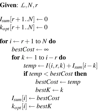
5. The Randomized Variable Elimination Algorithm
Given:
L
,N,rIsum[r+1..N]←0
kopt[r+1..N]←0
for i←r+1 to N do bestCost←∞ for k←1 to i−r do
temp←I(i,r,k) +Isum[i−k]
if temp<bestCost then bestCost←temp bestK←k Isum[i]←bestCost
kopt[i]←bestK
Table 1: Algorithm for computing k and cost values.
A backward approach serves two purposes for this algorithm. First, backward elimination eases the problem of recognizing irrelevant or redundant variables. As long as a core set of relevant variables remains intact, removing other variables should not harm the performance of a learning algorithm. Indeed, the learner’s performance may increase as irrelevant features are removed from consideration. In contrast, variables whose relevance depends on the presence of other variables may have no noticeable effect when selected in a forward manner. Thus, mistakes should be recognized immediately via backward elimination, while good selections may go unrecognized by a forward selection algorithm.
The second purpose of backward elimination is to ease the process of selecting variables. If most variables in a problem are irrelevant, then a random selection of variables is naturally likely to uncover them. Conversely, a random selection is unlikely to turn up relevant variables in a forward search. Thus, the forward search must work harder to find each relevant variable than backward search does for irrelevant variables.
5.1 Algorithm
The algorithm begins by computing the values of kopt(i,r)for all r+1≤i≤n. Next it generates an
initial hypothesis based on all n input variables. Then, at each step, the algorithm selects kopt(n,r)
Given:
L
, n, r, tolerancecompute tables for Isum(i,r)and kopt(i,r)
h←hypothesis produced by
L
on n inputswhile n>r do k←kopt(n,r)
select k variables at random and remove them h0←hypothesis produced by
L
on n−k inputs if e(h0)−e(h)≤tolerance thenn←n−k h←h0 else
replace the selected k variables
Table 2: Randomized backward-elimination variable selection algorithm.
The structured search performed by RVE is easily distinguished from other randomized search methods. For example, genetic algorithms maintain a population of states in the search space and randomly mate the states to produce offspring with properties of both parents. The effect is an initially broad search that targets more specific areas as the search progresses. A wide variety of subsets are explored, but the cost of so much exploration can easily exceed the cost of a traditional greedy search. See Goldberg (1989) or Mitchell (1996) for detailed discussions on how genetic algorithms conduct search.
While GAs tend to drift through the search space based on the properties of individuals in the population, the LVF algorithm (Liu and Setino, 1996) samples the space of variable subsets uniformly. LVF selects both the size of each subset and the member variables at random. Although such an approach is not susceptible to “bad decisions” or local minima, the probability of finding a best or even good variable subset decreases exponentially as the number of irrelevant variables increases. Unlike RVE, LVF is a filtering method, which relies on the inconsistency rate (number of equivalent instances divided by number of total instances) in the data with respect to the selected variables.
5.2 A Simple Example
M(
L
,N) SingleRVENumber of Input Variables
T
o
ta
l
U
p
d
ate
s
(
×
1
0
9)
500 450 400 350 300 250 200 150 100 50
30
25
20
15
10
5
0
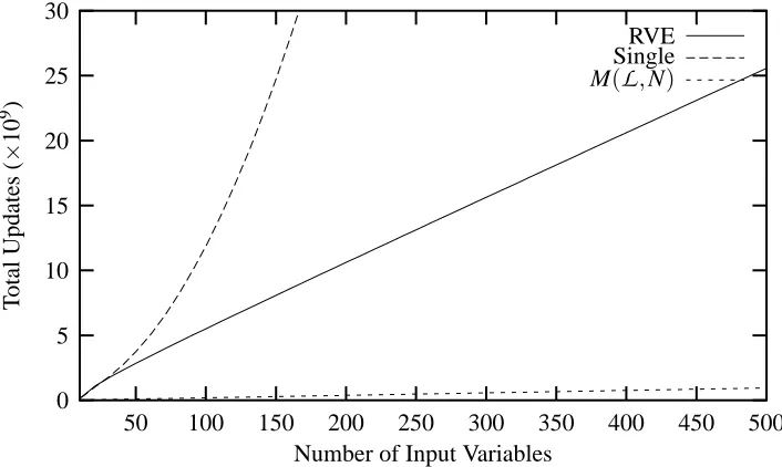
Figure 1: Plot of the expected cost of running RVE (Isum(N,r=10)) along with the cost of removing
inputs individually, and the estimated number of updates M(
L
,N).Twenty problems were generated randomly with N =100 input variables, of which 90 are ir-relevant and r=10 are relevant. Each of the twenty problems used a different set of ten relevant variables (selected at random) and different data sets. Two data sets, each with 1000 instances, were generated independently for each problem. One data set was used for training while the other was used to validate the error of the hypotheses generated during each round of selections. The values of the 100 input variables were all generated independently. The mean number of unique instances with respect to the ten relevant variables was 466 .
The first step in applying the RVE algorithm is to define the cost metric and the function M(
L
,n) for learning on n inputs. For the perceptron, we choose the number of weight updates as the metric. The thermal perceptron anneals a temperature T that governs the magnitude of the weight updates. Here we used T0=2 and decayed the temperature at a rate of 0.999 per training epoch until T<0.3 (we observed no change in the hypotheses produced by the algorithm for T <0.3). Given the tem-perature and decay rate, exactly 1897 training epochs are performed each time a thermal perceptron is trained. With 1000 instances in the training data, the cost of running the learning algorithm is fixed at M(L
,n) =1897000(n+1). Given the above cost formula for an n-input perceptron, a table of values for Isum(n,r)and kopt(n,r)can be constructed.After creating the table kopt(n,r), the selection and removal process begins. Since the
seven-of-ten learning problem is linearly separable, the tolerance for comparing the new and current hy-potheses was set to near zero. A small tolerance of 0.06 (equivalent to about 15 misclassifications) is necessary since the thermal perceptron does not guarantee a minimum error hypothesis.
We also allow the current hypothesis to bias the next by not randomizing the weights (of remain-ing variables) after each pass of RVE. Small value weights, suggestremain-ing potential irrelevant variables, can easily transfer from one hypothesis to the next, although this is not guaranteed. Seeding the per-ceptron weights may increase the chance of finding a linear separator if one exists. If no separator exists, then seeding the weights should have minimal impact. In practice we found that the effect of seeding the weights was nullified by the pocket perceptron’s use of annealing.
5.3 Example Results
The RVE algorithm was run using the twenty problems described above. Hypotheses based on ten variables were produced using an average of 5.45×10⁹ weight updates, 81.1 calls to the learning algorithm, and 359.9 seconds on a 3.12 GHz Intel Xenon processor. A version of the RVE algorithm that removes variables individually (i.e. k was set permanently to 1) was also run, and produced hypotheses using 12.7×10⁹ weight updates, 138.7 calls to the learner, and 644.7 seconds. These weight update values agree with the estimate produced by the cost function. Both versions of the algorithm generated hypotheses that included irrelevant and excluded relevant variables for three of the test problems. All cases in which the final selection of variables was incorrect were preceded by an initial hypothesis (based on all 100 variables) with unusually high error (error greater than 0.18 or approximately 45 misclassified instances). Thus, poor selections occured for runs in which the first hypothesis produced has high error due to annealing in the pocket perceptron.
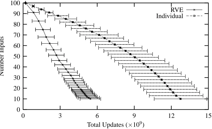
Figure 2 plots the average number of inputs used for each variable set size (number of inputs) compared to the total number of weight updates. Each marked point on the plot denotes a size of the set of input variables given to the perceptron. The error bars indicate the standard deviation in number of updates required to reach that point. Every third point is plotted for the individual removal algorithm. Compare both the rate of drop in inputs and the number of hypotheses trained for the two RVE versions. This reflects the balance between the cost of training and unsuccessful variable selections. Removing variables individually in the presence of many irrelevant variables ignores the cost of training each hypothesis, resulting in a total cost that rises quickly early in the search process.
6. Choosing k When r Is Unknown
The assumption that the number of relevant variables r is known has played a critical role in the preceding discussion. In practice, this is a strong assumption that is not easily met. We would like an algorithm that removes irrelevant attributes efficiently without such knowledge. One approach would be simply to guess values for r and see how RVE fares. This is unsatisfying however, as a poor guess can destroy the efficiency of RVE. In general, guessing specific values for r is difficult, but placing a loose bound around r may be much easier. In some cases, the maximum value for r may be known to be much less than N, while in other cases, r can always be bounded by 1 and N.
Given some bound on the maximum rmax and minimum rmin values for r, a binary search for
Individual RVE
Total Updates (×109)
N
u
mb
er
In
p
u
ts
15 12
9 6
3 0
100
90
80
70
60
50
40
30
20
10
0
Figure 2: A comparison between the number of inputs on which the perceptrons are trained and the mean aggregate number of updates performed by the perceptrons.
At each step of RVE, a certain number of failures, E−(n,r,k), are expected. Thus, if selecting variables for removal is too easy (i.e. we are selecting too few variables at each step), then the estimate for r is too high. Similarly, if selection fails an inordinate number of times, then the estimate for r is too low.
The choice of when to adjust r is important. The selection process must be allowed to fail a certain number of times for each success, but allowing too many failures will decrease the efficiency of the algorithm. We bound the number of failures by c1E−(n,r,k) where c1>1 is a constant. This allows for the failures prescribed by the cost function along with some amount of “bad luck” in the random variable selections. The number of consecutive successes is bounded similarly by c2(r−E−(n,r,k)) where c2 >0 is a constant. Since E−(n,r,k)) is at most r, the value of this expression decreases as the expected number of failures increases. In practice c1=3 and c2=0.3 appear to work well.
6.1 A General Purpose Algorithm
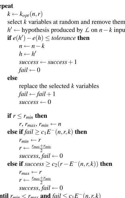
Randomized variable elimination including a binary search for r (RVErS — “reverse”) begins by computing tables for kopt(n,r)for values of r between rminand rmax. Next an initial hypothesis is
generated and the variable selection loop begins. The algorithm chooses the number of variables to remove at each step based on the current value of r. Each time the bound on the maximum number of successful selections is exceeded, rmax reduces to r and a new value is calculated as
r= rmax+rmin
Given:
L
, c1, c2, n, rmax, rmin, tolerancecompute tables Isum(i,r)and kopt(i,r)for rmin≤r≤rmax
r← rmax+rmin
2
success, f ail←0
h←hypothesis produced by
L
on n inputsrepeat
k←kopt(n,r)
select k variables at random and remove them h0←hypothesis produced by
L
on n−k inputs if e(h0)−e(h)≤tolerance thenn←n−k h←h0
success←success+1 fail←0
else
replace the selected k variables fail←fail+1
success←0
if r≤rminthen
r, rmax, rmin←n
else if fail≥c1E−(n,r,k)then rmin←r
r←rmax+rmin
2
success, fail←0
else if success≥c2(r−E−(n,r,k))then rmax←r
r←rmax+rmin
2
success, fail←0
until rmin<rmaxand fail≤c1E−(n,r,k)
Table 3: Randomized variable elimination algorithm including a search for r.
terminates when rminand rmaxconverge and c1E−(n,r,k)consecutive variable selections fail. Table
3 shows the RVErS algorithm.
Algorithm Mean Updates Mean Time (s) Mean Calls Mean Inputs
RVE (kopt) 5.5×10⁹ 359.9 81.1 10.0
rmax=20 6.5×10⁹ 500.7 123.8 10.8
rmax=40 8.0×10⁹ 603.8 151.3 10.2
rmax=60 9.3×10⁹ 678.8 169.0 10.0
rmax=80 10.0×10⁹ 694.7 172.3 10.0
rmax=100 11.7×10⁹ 740.7 184.1 9.9
RVE (k=1) 12.7×10⁹ 644.7 138.7 10.0
Table 4: Results of RVE and RVErS for several values of rmax. Mean calls refers to the number
calls made to the learning algorithm. Mean inputs refers to the number of inputs used by the final hypothesis.
With respect to the analysis presented in Section 4.2.1, note that the constants c1and c2do not impact the total cost of performing variable selection. However, a large number of adjustments to rminand rmaxdo impact the total cost negatively.
6.2 An Experimental Comparison of RVE and RVErS
The RVErS algorithm was applied to the seven-of-ten problems using the same conditions as the experiments with RVE. Table 4 shows the results of running RVErS based on five values of rmaxand
rmin=2. The results show that for increasing values of rmax, the performance of RVErS degrades
slowly with respect to cost. The difference between RVErS with rmax=100 and RVE with k=1
is significant at the 95% confidence level (p=0.049), as is the difference between RVErS with rmax=20 and RVE with k=kopt (p=0.0005). However, this slow degradation does not hold in
terms of run time or number of calls to the learning algorithm. Here, only versions of RVErS with rmax=20 or 40 show an improvement over RVE with k=1.
The RVErS algorithm termination criteria causes the sharp increase in the number of calls to the learning algorithm. Recall that as n approaches r the probability of a failed selection increases. This means that the number of allowable selection failures grows as the algorithm nears completion. Thus, the RVErS algorithm makes many calls to the learner using a small number of inputs n in an attempt to determine whether the search should be terminated. The search for r compounds the effect. If, at the end of the search, the irrelevant variables have been removed but rminand rmaxhave
not converged, then the algorithm must work through several failed sequences in order to terminate.
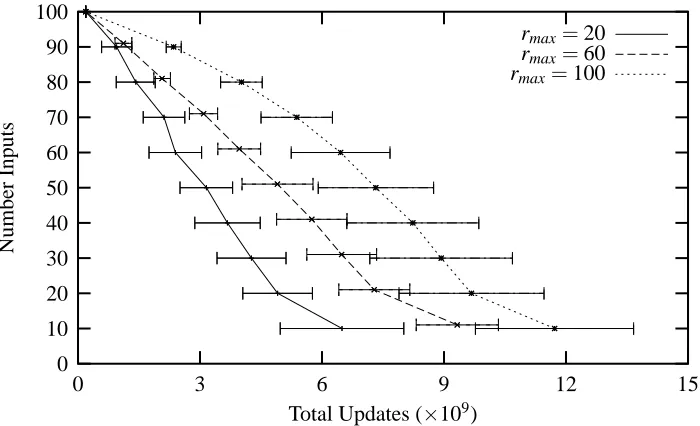
Figure 3 plots of the number of variables selected compared to the average total number of weight updates for rmax=20, 60 and 100. The error bars represent the standard deviation in the
rmax=100
rmax=60
rmax=20
Total Updates (×109)
N
u
mb
er
In
p
u
ts
15 12
9 6
3 0
100
90
80
70
60
50
40
30
20
10
0
Figure 3: A comparison between the number of inputs on which the thermal perceptrons are trained and the aggregate number of updates performed using the RVErS algorithm.
The increase in run times follows directly from the increasing number of calls to the learner. The thermal perceptron algorithm carries a great deal of overhead not reflected by the number of updates. Since the algorithm executes for a fixed number of epochs, the run time of any call to the learner will contribute noticeably to the run time of RVErS, regardless of the number of selected variables. Contrast this behavior to that of learner whose cost is based more firmly on the number of input variables, such as naive Bayes. Thus, even though RVErS always requires fewer weight updates than RVE with k=1, the latter may still run faster.
This result suggests that the termination criterion of the RVErS algorithm is flawed. The large number of calls to the learner at the end of the variable elimination process wastes a portion of the advantage generated earlier in the search. More importantly, the excess number of calls to the learner does not respect the very careful search trajectory computed by the cost function. Although our cost function for the learner M(
L
,n) does take the overhead of the thermal perceptron algorithm into account, there is no allowance for unnecessary calls to the learner. Future research with randomized variable elimination should therefore include a better termination criterion.7. Experiments with RVErS
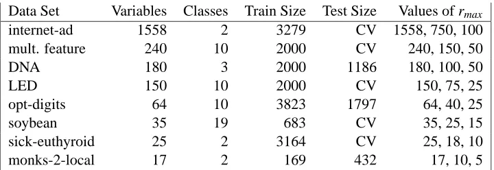
Data Set Variables Classes Train Size Test Size Values of rmax
internet-ad 1558 2 3279 CV 1558, 750, 100
mult. feature 240 10 2000 CV 240, 150, 50
DNA 180 3 2000 1186 180, 100, 50
LED 150 10 2000 CV 150, 75, 25
opt-digits 64 10 3823 1797 64, 40, 25
soybean 35 19 683 CV 35, 25, 15
sick-euthyroid 25 2 3164 CV 25, 18, 10
monks-2-local 17 2 169 432 17, 10, 5
Table 5: Summary of data sets.
Unlike the linearly-separable perceptron experiments, the problems used here do not necessarily have solutions with zero test error. The learning algorithms may produce hypotheses with more variance in accuracy, requiring a more sophisticated evaluation function. The utility of variable selection with respect to even the most sophisticated learning algorithms is well known, see for example Kohavi and John (1997) or Weston, Mukherjee, Chapelle, Pontil, Poggio, and Vapnik (2000). The goal here is to show that our comparatively liberal elimination method sacrifices little in terms of accuracy and gains much in terms of speed.
7.1 Learning Algorithms
The RVErS algorithm was applied to two learning algorithms. The first is the C4.5 release 8 algo-rithm (Quinlan, 1993) for decision tree induction with options to avoid pruning and early stopping. We avoid pruning and early stopping because these are forms of variable selection, and may obscure the performance of RVErS. The cost metric for C4.5 is based on the number of calls to the gain-ratio data purity criterion. The cost of inducing a tree is therefore roughly quadratic in the number of variables: one call per variable, per decision node, with at most a linear number of nodes in the tree. Recall that an exact metric is not needed, only the order with respect to the number of variables must be correct.
The second learning algorithm used is naive Bayes, implemented as described by Mitchell (1997). Here, the cost metric is based on the number of operations required to build the condi-tional probability table, and is therefore linear in the number of inputs. In practice, these tables need not be recomputed for each new selection of variables, as the irrelevant table entries can simply be ignored. However, we recompute the tables here to illustrate the general case in which the learning algorithm must start from scratch.
7.2 Data Sets
are possible, but not instructive, as randomized elimination is not intended for data sets with few variables.
Three of the data sets (DNA, opt-digits, and monks) include predetermined training and test sets. The remaining problems used ten-fold cross validation. The version of the LED problem used here was generated using code available at the repository, and includes a corruption of 10% of the class labels. Following Kohavi and John, the monks-2 data used here includes a local (one of n) encoding for each of the original six variables for a total of 17 Boolean variables. The original monks-2 problem contains no irrelevant variables, while the encoded version contains six irrelevant variables.
7.3 Methodology
For each data set and each of the two learning algorithms (C4.5 and naive Bayes), we ran four versions of the RVErS algorithm. Three versions of RVErS use different values of rmaxin order to
show how the choice of rmaxaffects performance. The fourth version is equivalent to RVE with k=1
using a stopping criterion based on the number of consecutive failures (as in RVErS). This measures the performance of removing variables individually given that the number of relevant variables is completely unknown. For comparison, we also ran forward step-wise selection, backward step-wise elimination and a hybrid filtering algorithm. The filtering algorithm simply ranked the variables by gain-ratio, executed the learner using the first 1, 2, 3,. . ., N variables, and selected the best.
The learning algorithms used here provide no performance guarantees, and may produce highly variable results depending on variable selections and available data. All seven selection algorithms therefore perform five-fold cross-validation using the training data to obtain an average hypothesis accuracy generated by the learner for each selection of variables. The methods proposed by Kohavi and John (1997) could be used to improve error estimates for cases in which the variance in hypoth-esis error rates is high. Their method should provide reliable estimates for adjusting the values of rminand rmaxregardless of learning algorithm.
Preliminary experiments indicated that the RVErS algorithm is more prone to becoming bogged down during the selection process than deterministic algorithms. We therefore set a small tolerance (0.002) as shown in Table 3, which allows the algorithm to keep only very good selections of vari-ables while still preventing the selection process from stalling unnecessarily. We have not performed extensive tests to determine ideal tolerance values.
The final selections produced by the algorithms were evaluated in one of two ways. Domains for which there no specific test set is provided were evaluated via ten-fold cross-validation. The remaining domains used the provided training and test sets. In the second case, we ran each of the four RVErS versions five times in order to smooth out any fluctuations due to the random nature of the algorithm.
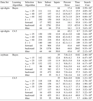
7.4 Results
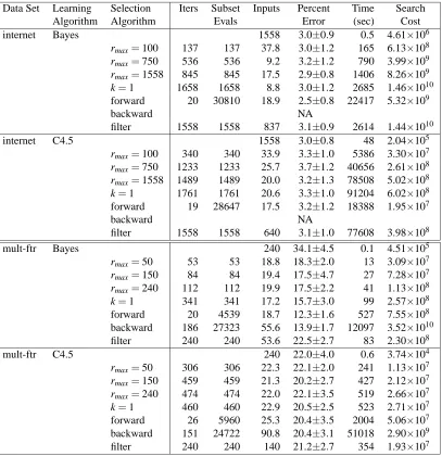
Data Set Learning Selection Iters Subset Inputs Percent Time Search
Algorithm Algorithm Evals Error (sec) Cost
internet Bayes 1558 3.0±0.9 0.5 4.61×10⁶
rmax=100 137 137 37.8 3.0±1.2 165 6.13×10⁸ rmax=750 536 536 9.2 3.2±1.2 790 3.99×10⁹ rmax=1558 845 845 17.5 2.9±0.8 1406 8.26×10⁹ k=1 1658 1658 8.8 3.0±1.2 2685 1.46×10¹⁰ forward 20 30810 18.9 2.5±0.8 22417 5.32×10⁹
backward NA
filter 1558 1558 837 3.1±0.9 2614 1.44×10¹⁰
internet C4.5 1558 3.0±0.8 48 2.04×10⁵
rmax=100 340 340 33.9 3.3±1.0 5386 3.30×10⁷ rmax=750 1233 1233 25.7 3.7±1.2 40656 2.61×10⁸ rmax=1558 1489 1489 20.0 3.2±1.3 78508 5.02×10⁸ k=1 1761 1761 20.6 3.3±1.0 91204 6.02×10⁸ forward 19 28647 17.5 3.2±1.2 18388 1.95×10⁷
backward NA
filter 1558 1558 640 3.1±1.0 77608 3.98×10⁸
mult-ftr Bayes 240 34.1±4.5 0.1 4.51×10⁵
rmax=50 53 53 18.8 18.3±2.0 13 3.09×10⁷ rmax=150 84 84 19.4 17.5±4.7 27 7.28×10⁷ rmax=240 112 112 19.9 17.5±2.2 41 1.13×10⁸ k=1 341 341 17.2 15.7±3.0 99 2.57×10⁸ forward 20 4539 18.7 12.3±1.6 527 7.55×10⁸
backward 186 27323 55.6 13.9±1.7 12097 3.52×10¹⁰ filter 240 240 53.6 22.5±2.7 83 2.30×10⁸
mult-ftr C4.5 240 22.0±4.0 0.6 3.74×10⁴
rmax=50 306 306 22.3 22.1±2.0 241 1.13×10⁷ rmax=150 459 459 21.3 20.2±2.7 427 2.12×10⁷ rmax=240 474 474 22.0 22.1±3.5 519 2.66×10⁷ k=1 460 460 22.9 20.5±2.5 523 2.71×10⁷
forward 26 5960 25.3 20.4±3.5 2004 5.06×10⁷ backward 151 24722 90.8 20.4±3.1 51018 2.90×10⁹ filter 240 240 140 21.2±2.7 354 1.93×10⁷
Table 6: Variable selection results using the naive Bayes and C4.5 learning algorithms.
the performance of the seven selection algorithms. Finally, “NA” indicates that the experiment was terminated due to excessive computational cost.
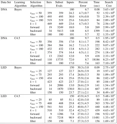
Data Set Learning Selection Iters Subset Inputs Percent Time Search
Algorithm Algorithm Evals Error (sec) Cost
DNA Bayes 180 6.7 0.08 3.63×10⁵
rmax=50 359 359 24.2 4.7±0.7 52 1.52×10⁸ rmax=100 495 495 30.0 4.9±0.8 75 2.39×10⁸ rmax=180 519 519 25.6 5.0±0.5 84 2.89×10⁸ k=1 469 469 23.6 4.7±0.3 76 2.56×10⁸ forward 19 3249 18.0 5.8 269 2.99×10⁸ backward 34 5413 148 6.5 1399 7.16×10⁹
filter 180 180 101 5.7 32 1.33×10⁸
DNA C4.5 180 9.7 0.5 1.95×10⁴
rmax=50 356 356 17.0 8.1±1.7 198 8.42×10⁶ rmax=100 384 384 16.2 7.1±1.5 222 9.07×10⁶ rmax=180 432 432 13.8 6.5±1.2 282 1.21×10⁷ k=1 374 374 14.4 6.5±1.1 274 1.18×10⁷
forward 13 2262 12.0 5.9 418 2.33×10⁶ backward 110 13735 72.0 8.7 18186 8.23×10⁸ filter 180 180 17.0 7.6 163 7.10×10⁶
LED Bayes 150 30.3±3.0 0.09 2.75×10⁵
rmax=25 127 127 22.7 26.9±3.9 19 3.97×10⁷ rmax=75 293 293 17.4 26.0±3.3 50 1.09×10⁸ rmax=150 434 434 25.6 25.9±2.6 86 2.02×10⁸ k=1 423 423 23.7 27.0±2.1 85 2.04×10⁸ forward 14 2006 13.0 26.6±2.9 141 1.54×10⁸
backward 14 1870 138.0 30.1±2.6 667 1.95×10⁹ filter 150 150 23.7 27.1±2.1 34 8.49×10⁷
LED C4.5 150 43.9±4.5 0.5 5.48×10⁴
rmax=25 85 85 51.1 42.0±3.0 89 1.01×10⁷ rmax=75 468 468 25.8 42.5±4.5 363 3.70×10⁷ rmax=150 541 541 25.2 40.8±5.7 440 4.48×10⁷ k=1 510 510 32.4 42.5±2.7 439 4.63×10⁷
forward 9 1286 7.8 27.0±3.2 196 9.52×10⁵ backward 61 7218 90.9 43.5±3.5 11481 1.33×10⁹ filter 150 150 7.1 27.3±3.5 156 1.69×10⁷
Table 7: Variable selection results using the naive Bayes and C4.5 learning algorithms.
The internet-ad via C4.5 experiment highlights a second point. Notice how the forward selection algorithm runs faster than all but one version of RVErS. In this case, the cost and time of running C4.5 many times on a small number of variables is less than that of running C4.5 few times on many variables. However, note that a slight change in the number of iterations needed by the forward algorithm would change the time and cost of the search dramatically. This is not the case for RVErS, since each iteration involves only a single evaluation instead of O(N)evaluations.
Addi-Data Set Learning Selection Iters Subset Inputs Percent Time Search
Algorithm Algorithm Evals Error (sec) Cost
opt-digits Bayes 64 17.4 0.08 2.59×10⁵
rmax=25 111 111 14.2 15.7±1.5 15.9 4.05×10⁷ rmax=40 157 157 13.2 14.9±0.7 22.9 5.92×10⁷ rmax=64 162 162 14.4 14.7±1.0 24.9 6.66×10⁷ k=1 150 150 14.0 14.2±1.1 24.7 6.76×10⁷ forward 17 952 16.0 14.1 93.8 1.91×10⁸ backward 41 1781 25.0 13.5 423.0 1.39×10⁹
filter 64 64 37.0 16.1 11.9 3.63×10⁷
opt-digits C4.5 64 43.2 0.7 2.15×10⁴
rmax=25 130 130 12.0 42.4±2.0 148 3.64×10⁶ rmax=40 158 158 10.8 42.2±0.3 181 4.42×10⁶ rmax=64 216 216 10.4 42.5±1.2 253 6.36×10⁶ k=1 140 140 11.4 42.1±1.1 189 5.33×10⁶ forward 16 904 15.0 41.6 645 9.64×10⁶ backward 28 1378 38.0 44.0 2842 9.55×10⁷
filter 64 64 50.0 43.6 87 2.12×10⁶
soybean Bayes 35 7.8±2.4 0.02 2.40×10⁴
rmax=15 142 142 12.6 8.9±4.2 5.9 6.47×10⁶ rmax=25 135 135 11.9 10.5±5.8 5.8 6.26×10⁶ rmax=35 132 132 11.2 9.8±5.1 5.8 6.17×10⁶ k=1 88 88 12.3 9.6±5.0 4.6 4.67×10⁶ forward 13 382 12.3 7.3±2.9 8.9 1.09×10⁷ backward 19 472 18.0 7.9±4.6 37.5 3.63×10⁷
filter 35 35 31.3 7.8±2.6 2.0 1.97×10⁶
C4.5 35 8.6±4.0 0.04 1.21×10³
rmax=15 118 118 16.3 9.5±4.6 13.5 2.78×10⁵ rmax=25 158 158 14.7 10.1±4.1 18.6 1.90×10⁵ rmax=35 139 139 16.3 9.1±3.7 17.3 3.86×10⁵ k=1 117 117 16.1 9.3±3.5 14.9 3.52×10⁵ forward 16 435 14.8 9.1±4.0 33.7 3.22×10⁵ backward 18 455 19.1 10.4±4.4 69.0 1.75×10⁶ filter 35 35 30.8 8.5±3.7 3.7 6.06×10⁴
Table 8: Variable selection results using the naive Bayes and C4.5 learning algorithms.
tional tests using data with many hundreds or thousands of variables would be instructive, but may not be feasible with respect to the deterministic search algorithms.
RVErS does not achieve the same economy of subset evaluations on the three smaller problems as on the larger problems. This is not surprising, since the ratio of relevant variables to total variables is much smaller, requiring RVErS to proceed more cautiously. In these cases, the value of rmaxhas
only a minor effect on performance, as RVErS is unable to remove more than two or three variables in any given step.
Data Set Learning Selection Iters Subset Inputs Percent Time Search
Algorithm Algorithm Evals Error (sec) Cost
euthyroid Bayes 25 6.2±1.3 0.02 7.54×10⁴
rmax=10 30 30 2.0 4.6±1.5 2.1 2.65×10⁶ rmax=18 39 39 2.0 4.8±1.2 1.3 3.73×10⁶ rmax=25 46 46 2.3 5.1±1.4 1.6 4.32×10⁶ k=1 35 35 1.7 5.0±1.2 1.5 4.86×10⁶
forward 5 118 4.2 4.6±1.1 3.4 6.45×10⁶ backward 16 263 11.3 4.2±1.3 14.4 5.91×10⁷ filter 25 25 4.7 4.2±0.6 1.4 4.16×10⁶
C4.5 25 2.7±1.0 0.2 1.00×10³
rmax=10 49 49 2.9 2.4±0.8 21.0 2.98×10⁴ rmax=18 63 63 3.3 2.2±0.7 27.6 4.58×10⁴ rmax=25 55 55 2.7 2.5±0.8 25.3 4.92×10⁴ k=1 54 54 3.8 2.3±0.9 29.4 6.39×10⁴ forward 7 151 5.9 2.4±0.7 51.8 3.89×10⁴ backward 16 269 11.0 2.5±0.9 200.0 6.73×10⁵
filter 25 25 15.2 2.7±1.1 15.4 3.60×10⁴
monks-2 Bayes 17 39.4 0.01 3.11×10³
rmax=5 25 25 2.6 36.1±3.2 0.02 1.10×10⁵ rmax=10 54 54 4.0 37.2±2.3 0.05 2.50×10⁵ rmax=17 74 74 6.0 37.4±3.1 0.08 4.93×10⁵ k=1 41 41 6.0 36.8±3.1 0.04 2.89×10⁵
forward 2 33 1.0 32.9 0.02 6.70×10⁴
backward 8 99 11.0 38.4 0.13 9.93×10⁵
filter 17 17 2.0 40.3 0.01 1.21×10⁵
C4.5 17 23.6 0.03 5.14×10²
rmax=5 36 36 8.2 16.7±10.9 0.8 2.34×10⁴ rmax=10 84 84 6.2 4.6±0.4 1.9 3.74×10⁴ rmax=17 79 79 6.4 6.5±4.7 1.8 4.63×10⁴ k=1 55 55 6.2 4.4±0.0 1.4 4.13×10⁴
forward 2 33 1.0 32.9 0.6 3.95×10²
backward 13 139 6.0 4.4 3.9 1.61×10⁵
filter 17 17 13.0 35.6 0.4 1.51×10⁴
Table 9: Variable selection results using the naive Bayes and C4.5 learning algorithms.
but there are exceptions. In some cases, rmaxhas very little effect on error. However, in most cases,
small values of rmaxhave a distinct positive effect on run time.
3.5 4 4.5 5 5.5 6 6.5 7
0 50 100 150 200 250 300 350
Error
Iterations RVErS rmax=50
Test CV 4 4.5 5 5.5 6 6.5 7
0 50 100 150 200 250 300 350 400
Error
Iterations RVErS rmax=100
Test CV 3.5 4 4.5 5 5.5 6 6.5 7
0 100 200 300 400 500
Error
Iterations RVErS rmax=180
Test CV 4 4.5 5 5.5 6 6.5 7
0 50 100 150 200 250 300 350 400
Error
Iterations RVErS k=1
Test CV 0 5 10 15 20 25 30 35 40
0 2 4 6 8 10 12 14 16 18
Error Iterations Forward Test CV 4 4.5 5 5.5 6 6.5 7
0 5 10 15 20 25 30 35
Error
Iterations Backward
Test CV
6 7 8 9 10 11 12 13
0 50 100 150 200 250 300 350 400
Error
Iterations RVErS rmax=50
Test CV 6.5 7 7.5 8 8.5 9 9.5 10 10.5
0 50 100 150 200 250 300
Error
Iterations RVErS rmax=100
Test CV 5 6 7 8 9 10 11
0 50 100 150 200 250 300 350
Error
Iterations RVErS rmax=180
Test CV 6 6.5 7 7.5 8 8.5 9 9.5 10 10.5
0 50 100 150 200 250 300
Error
Iterations RVErS k=1
Test CV 0 5 10 15 20 25 30 35 40
0 2 4 6 8 10 12
Error Iterations Forward Test CV 4 5 6 7 8 9 10 11
0 20 40 60 80 100 120
Error
Iterations Backward
Test CV
Overfitting is sometimes a problem with greedy variable selection algorithms. Figures 4 and 5 show both the test and inner (training) cross-validation error rates for the selection algorithms on naive Bayes and C4.5 respectively. Solid lines indicate test error, while dashed lines indicate the inner cross-validation error. Notice that the test error is not always minimized with the final selections produced by RVErS. The graphs show that RVErS does tend to overfit naive Bayes, but not C4.5 (or at least to a lesser extent). Trace data from the other data sets agree with this conclusion. There are at least two possible explanations for overfitting by RVErS. One is that the tolerance level either causes the algorithm to continue eliminating variables when it should stop, or allows elimination of relevant variables. In either case, a better adjusted tolerance level should improve performance. The monks-2 data set provides an example. In this case, if the tolerance is set to zero, RVErS reliably finds variable subsets that produce low-error hypotheses with C4.5.
A second explanation is that the stopping criteria, which becomes more difficult to satisfy as the algorithm progresses, causes the elimination process to become overzealous. In this case the solution may be to augment the given stop criteria with a hold-out data set (in addition to the vali-dation set). Here the algorithm monitors performance in addition to counting consecutive failures, returning the best selection, rather than simply the last. Combining this overfitting result with the above performance results suggests that RVErS is capable of performing quite well with respect to both generalization and speed.
8. Discussion
The speed of randomized variable elimination stems from two aspects of the algorithm. One is the use of large steps in moving through the search space of variable sets. As the number of irrelevant variables grows, and the probability of selecting a relevant variable at random shrinks, RVE attempts to take larger steps toward its goal of identifying all of the irrelevant variables. In the face of many irrelevant variables, this is a much easier task than attempting to identify the relevant variables.
The second source of speed in RVE is the approach of removing variables immediately, instead of finding the best variable (or set) to remove. This is much less conservative than the approach taken by step-wise algorithms, and accounts for much of the benefit of RVE. In practice, the full benefit of removing multiple variables simultaneously may only be beginning to materialize in the data sets used here. However, we expect that as domains scale up, multiple selections will become increasingly important. One example of this occurs in the STL algorithm (Utgoff and Stracuzzi, 2002), which learns many concepts over a period of time. There, the number of available input variables grows as more concepts are learned by the system.
Consider briefly the cost of forward selection wrapper algorithms. Greedy step-wise search is bounded by O(rNM(