Query Transformations for Improving the Efficiency of ILP Systems
V´ıtor Santos Costa [email protected]
COPPE/Sistemas, UFRJ, Brazil and LIACC, Universidade do Porto, Portugal
Ashwin Srinivasan [email protected] Oxford University Computing Laboratory
Wolfson Bldg., Parks Rd, Oxford, UK
Rui Camacho [email protected]
LIACC and FEUP, Universidade do Porto, Portugal
Hendrik Blockeel [email protected]
Bart Demoen [email protected]
Gerda Janssens [email protected]
Jan Struyf [email protected]
Department of Computer Science, Katholieke Universiteit Leuven, Celestijnenlaan 200A, B-3001, Leuven, Belgium
Henk Vandecasteele [email protected] PharmaDM
Ambachtenlaan 54D, B-3001, Leuven, Belgium
Wim Van Laer [email protected]
Department of Computer Science, Katholieke Universiteit Leuven Celestijnenlaan 200A, B-3001, Leuven, Belgium
Editors: James Cussens and Alan M. Frisch
Abstract
Relatively simple transformations can speed up the execution of queries for data mining consider-ably. While some ILP systems use such transformations, relatively little is known about them or how they relate to each other. This paper describes a number of such transformations. Not all of them are novel, but there have been no studies comparing their efficacy. The main contributions of the paper are: (a) it clarifies the relationship between the transformations; (b) it contains an empiri-cal study of what can be gained by applying the transformations; and (c) it provides some guidance on the kinds of problems that are likely to benefit from the transformations.
Keywords: Inductive Logic Programming, Program Analysis
1. Introduction
Like many other algorithms in the field of machine learning, ILP algorithms construct “hy-potheses” for data by performing a search through a large space. Such a search typically involves generating and then testing the quality of candidates. Testing a candidate hypothesis involves exe-cuting a query in first-order logic against the data. Improvements in efficiency thus result from (A) minimizing, to the best extent possible, the number of candidates generated; and (B) maximizing, to the best extent possible, the efficiency of testing each candidate.
Problem (A)—minimizing the search space—has received a lot of attention in ILP research. This has resulted in the development of powerful language bias specification mechanisms that limit the size of the search space (N´edellec et al., 1996) the study of refinement operators that allow one to efficiently navigate through a hypothesis space (van der Laag and Nienhuys-Cheng, 1998), etc.
Problem (B)—efficient testing of candidate hypotheses—does not appear to have received as much attention. It is the less pressing problem: however, in the light of the advances that have been made on techniques for minimizing the search space, the issue does become important. There has been some previous work of a stochastic nature (Srinivasan, 1999; Sebag and Rouveirol, 1997). These reduce the evaluation effort at the cost of being correct only with high probability. This paper is concerned with exact transformations, extending the work first reported by Santos Costa et al. (2000). In that paper, the authors illustrated that query execution was a very high percentage of total running time. They also proposed two simple transformations that converted a first order query into an equivalent one which was more efficient to execute. Empirical evidence presented suggested that under some conditions the transformations could significantly improve the efficiency of an ILP system—there, the system Aleph (Srinivasan, 2001). Here, we extend this work in the following ways: (1) we consider two further transformations; (2) we describe how the four transformations relate to each other; (3) we present a theoretical analysis of the transformations; and (4) we provide empirical evidence of the behaviour of the transformations on artificial and real-world problems.
The paper is organised as follows: in Section 2 we outline a simple procedure that serves as a model for many ILP algorithms. Section 3 describes the four transformations. Section 4 provides an analysis of the computational complexity of the transformations as well as the execution of the original and transformed queries. An empirical evaluation of the approach is presented in Section 5. Section 6 concludes the paper. The paper is accompanied by two appendices containing material relevant to Sections 3 and 5.
2. A Simple ILP Implementation
We adopt the following informal prescription for an ILP algorithm, based on Muggleton (1994). We are given: (a) background knowledge B in the form of a Prolog program; (b) some language specification
L
describing the hypothesis space; (c) an optional set of constraints I on acceptable hypotheses; and (d) a finite set of examples E such that none of the elements of set E are derivable from B. The set is divided into a set of positive examples E+and a set of negative examples E−. The task is to find some hypothesis H ∈L
such that (1) H is consistent with the I; (2) the E+ are derivable from B∪H; and (3) the E−are not derivable from B∪H.generalise(B,I,
L
,E): Given background knowledge B, hypothesis constraints I, a finite training set E=E+∪E−, returns a hypothesis H inL
such that B∪H derives the E+.1. i=0
2. Ei+=E+, Hi=/0 3. while Ei+6=/0do
(a) increment i
(b) Traini=Ei−+1∪E−
(c) Di=search(B,Hi−1,I,
L
,Traini) (d) Hi=Hi−1∪ {Di}(e) Ep={ep: ep∈Ei+−1s.t.B∪Hi|={ep}}. (f) Ei+=Ei+−1\Ep
4. return Hi
Figure 1: A simple ILP implementation. The function search() is some search procedure that re-turns one clause after evaluating alternatives in some search-space of clauses, all of which are in
L
.A1. On each iteration, search() will examine a finite number of clauses;
A2. For each clause examined, search() will check (at least) the derivability of each example in Traini;
A3. The check for derivability always terminates; and
A4. The actual proofs of derivability of an example are irrelevant to evaluating the ‘goodness’ of a clause.
These assumptions hold not only for ILP systems that use an algorithm similar to the one in Figure 1, but for a much broader range of relational learning systems, including systems that induce trees, e.g. SRT (Kramer, 1996), instance based learners e.g. RIBL (Emde and Wettschereck, 1996) etc. Our results are equally relevant for those approaches. The transformations we propose in the next section are concerned with improving the efficiency of derivation checks arising from Assumption A2.
3. Four Query Transformations
All the transformations we study are ‘correct’ in the following sense: if a clause Di is transformed into a clause D0i, then B∪Hi−1∪{Di0}derives exactly the same examples in Trainias B∪Hi−1∪{Di}. If Assumption A4 holds, the identification of the best clause by search() will then be unaffected.
3.1 The Theta-transformation tθ
We are concerned here with clauses of the form Head :−Body where Body is a conjunction of goals G1,...,Gn (in the Prolog sense, or literals in the more traditional logical sense). Each of the Gi are meta-calls to user-defined or built-in predicates. In general, let N be an upper-bound on the number of solutions to any of the Gi. It follows straightforwardly that in the worst-case, the number of meta-calls is O(Nn). Lowering N requires a re-appraisal of predicate definitions used by clauses (either by re-encoding of some predicates, or by removing them entirely). We do not pursue this here, and concentrate instead on lowering the value of n.
A straightforward reduction in the number of goals being tested (thus lowering n) is achieved by eliminating obviously redundant ones. A simple logical check for this during the execution of the steps described in Figure 1 is as follows. On iteration i of the procedure in Figure 1, let P denote B∪Hi−1. Let C be a clause being examined in a search. Then, a literal l in C is redundant iff P∪{C} is logically equivalent with P∪ {C0}where C0=C− {l}.
From this, it is easy to show that l is redundant iff P∪ {C} |={C0}. This constraint, while providing an exact test for literal-redundancy, is expensive to implement (with a resolution-based theorem prover like that in YAP, it requires checking for the proof of inconsistency from the set P∪ {C}∪{¬C0}). Instead, we will employ a simpler test based on the subsumption relation (Nienhuys-Cheng and De Wolf, 1997). Recall that C subsumes C0 iff there is some substitution θsuch that Cθ⊆C0and if C subsumes C0then{C} |={C0}. Clearly therefore if C subsumes C0then P∪{C} |= {C0}and l is redundant (the reverse is not true, and hence we call it a “weak” test for redundancy).
We call the transformation that removes a set of redundant goals from a clause the Theta-transformation. It is evident that a transformation that removes redundant goals is correct. We use an approximation of the clausal-subsumption test (see Section 4) that is relatively inexpensive to perform and retains the property of correctness.1 While this is a simple transformation technique, it is not clear from descriptions of existing ILP systems whether they actually employ it during the search.2 In general, while the efficacy of the transformation will depend on the enumeration operator employed by the search function (that is, whether it is prone to introduction of redundant literals), we expect it to be more useful when the background predicates are non-determinate.
3.2 The Cut-transformation t!
We observe that when executing a conjunction of goals G1,...,Gn, failure of a goal Gi will result in attempting to generate more solutions for goals earlier in the sequence. This effort is useless if these solutions do not alter the computation of Gi. The cut-transformation, t!, exploits the notion of goal independence by partitioning the set of goals in a clause into classes such that goals in different classes are independent. We will execute each class in sequence, and use the pruning operator ! to avoid any backtracking between classes.
In pure logic programs, goals depend on each other because they share variables. Given a function vars(T)that returns all variables in the term T , two goals Giand Gjare said to share, that is the relation Shares(Gi,Gj)holds, when:
1. Significant work has been spent on correct and efficient implementations of subsumption tests (Kietz and L¨ubbe, 1994; Scheffer et al., 1996), but for the goals of this paper our simple implementation is good enough.
i=j ∨ vars(Gi)∩vars(Gj)6=/0
The definition ensures that the relation Shares is reflexive and symmetric. Its transitive closure Linked, defined as the smallest transitive relation that is a superset of Shares, is reflexive, symmetric and transitive, and therefore an equivalence relation.
Given a set of goals
G
={G1,...,Gn}, we shall name the equivalence classes established by Linked as I1,...,Im. If two goals are in the same equivalence class, we will say they may be de-pendent, otherwise we will say they are independent. We would like to divide the original clause into several conjunctions of independent goals and execute them separately.3 To do so, we place the goals in each class Iiin a conjunctionG
i. Our notion of dependence is a safe approximation of the dependencies that can possibly occur at run-time, because as soon as two goals have a variable in common they belong to the same equivalence class. Moreover, the computation of the equivalence classes is efficient.In this approximation all goals that include a head variable or that share variables with one such goal will belong to the same independence class. Often, we know beforehand that head variables will be grounded before calling the body. Clearly, such variables cannot introduce sharing. To take advantage of this extra information, we classify variables as either Grounded or PossiblySharing, and define vars(T) to return all PossiblySharing variables in T . More sophisticated analysis is possible, as discussed in Appendix A.
To effect t!it is sufficient to implement the following procedure: 1. Given the original clause:
H:- G1, ..., Gi, ..., Gn.
classify all variables in H,G1,...,Gnas Grounded or PossiblySharing and compute the equiv-alence classes for the (approximated) sharing relation.
2. Number the goal literals according to the equivalence class they belong to:
H:- G1 j, ..., Gik, ..., Gnl. 3. Reorder the literals in the clause according to the class they belong to:
H:- Ga1, ..., Gb1,..., Gcm, ..., Gdm.
4. We are interested in any solution, if one exists. Thus we need to compute every class once and if a class has no solution, the computation should wholly fail. The following program transformation usescutto guarantee such a computation:
H:- Ga1, ..., Gb1,!,...,!, Gcm, ..., Gdm.
The transformation is correct in the sense that the examples derivable before and after the trans-formation are the same. Step (3) is correct because the switching lemma allows us to reorder goals. Step (4) is correct because whenever we introduce a new cut, all goals before the cut are independent of all goals after the cut. Backtracking to before the cut therefore could never result in new solutions for the goals after the cut. A more complete discussion is given by Santos Costa et al. (2000).
3.3 The Once-transformation to
The cut transformation just described ensures that the search for each independent set of subgoals always stops at finding the first solution. Notice that the transformed body goal q1,!,q2,!,...,qncan also be written as once(q1),once(q2),...,once(qn) where the meta-predicateonceis defined as
once(X):- X, !.
While at the clause level theonceconstructs have the same effect as the cuts, they have the advan-tage that they can be nested, whereas cuts cannot.
The objective is to fine-tune t! by processing each set of independent goals in more detail. We start from the observation that the data guiding the successful application of the cut-transformation was that certain variables are known not to share at runtime. We can improve the partitioning process further by using extra data for each non-head variable and by taking advantage of Prolog’s left-to-right selection function. More precisely, we shall use prior knowledge on whether a literal grounds some of its arguments, and on whether a literal cannot cause its arguments to share by considering the status of each variable, as we move from goal to goal. This will allow us to transform each independent set of goals by considering the variables grounded by the first literal just like the ground head variables in the cut transformation. We then apply the transformation recursively and refine each independent set of subgoals into subsubsets.
Example 1 Consider the query p(X,Y,Z), q(X,Y,U), q(X,Z,V). If p grounds X and cannot cause
Y and Z to share, then q(X,Y,U) and q(X,Z,V) do not share, and after the call to p they can be executed independently.
We therefore ‘look inside’ each equivalence class returned by the t!. First, we find a prefix of one or more literals such that each literal will ground some of its arguments and it is known not to cause sharing among the others, then we apply the cut transformation on the rest of this subgoal, treating the grounded variables just like ground head variables.
We call this transformation the once-transformation or to. Blockeel et al. (2000b) describe two different versions of to. The dynamic version transforms queries during their execution, which results in an overhead but which also makes it possible to check groundness and sharing during execution instead of having to pre-compute a safe approximation. However, we only present the static version here.
once-transform(q): let q=l1,l2,...,ln
find the smallest k s.t. there exists a partition
P
of{lk+1,...,ln}s. t.∀qi,qj∈P
: V(qi)∩V(qj)⊆GroundedVars({l1,...,lk})and∀v∈V(qi),w∈V(qj):{v,w} 6∈PossiblySharing({l1,...,lk}) for all qi∈
P
: once-transform(qi)Figure 2: The once-transformation algorithm. GroundedVars(G) contains all variables grounded by a call to G. PossiblySharing(G) is the set of all pairs of variables that may share after a call to G.
A high level description of the once-transformation algorithm is shown in Figure 2. Essentially, the algorithm finds a prefix of a conjunction such that this prefix grounds enough variables for the rest of the conjunction to contain independent subgoals; then it is called recursively on these subgoals. Note that, similar to the cut transformation, we assume that the order of independent groups of literals may be switched but the relative order of literals that are dependent of each other does not change.
3.4 The Smartcall-transformation ts
The smartcall-transformation ts, called thus for historical reasons, was originally described by Bloc-keel (1998). The basic idea is as follows. ILP systems typically generate a clause by adding literals to (or refining) a clause encountered earlier (its parent). Assume a clause c=h← p,q has as parent h← p. The parent clause has been evaluated before, which means at some point it was computed which facts hθ are derived by the clause. If these θ are remembered, we can exploit this in two ways. Firstly, for the refined clause we need to check derivability of these facts only, because the facts derivable by the new clause are necessarily a subset of the examples derivable by its parent. Secondly, each derivability test can itself be simplified, and this is exactly what the smartcall-transformation does. Consider the equivalence classes Iiof c, as mentioned above. Each class can be checked independently of the others. For those Iifor which Ii⊆p, a solution must exist because there is one for the whole p. Hence, when testing the new clause with a head substitution
θ, we only need to check those Iithat contain literals that were added during refinement.
Example 2 Consider a clause P =p(X) :- a(X,Y), b(X,Z)to which during refinement a literal c(X,U)is added, resulting in
Q =p(X) :- a(X,Y), b(X,Z), c(X,U).
We have
t!(Q) =p(X) :- a(X,Y), !, b(X,Z), !, c(X,U).
If P is known to derive a specific fact p(e), we know that the goals a(e,Y)and b(e,Z)must have solutions. Moreover, c(e,U)can be checked independently from these goals. Hence, tscan drop the first two equivalence classes, yielding ts(Q) =p(X) :- c(X,U).
t!(Q0) =p(X) :- a(X,Y), c(X,Y), !, b(X,Z).
Now b(X,Z)can still be dropped, but a(X,Y)cannot, because even when we know the goal a(e,Y) has a solution, the conjunction(a(e,Y),c(e,Y)may not have any.
The smartcall-transformation is correct in the following sense : given that an example was de-rived by the parent clause, it can be dede-rived by the transformed clause if and only if it can be dede-rived by the original clause. The emphasized condition need not be fulfilled for the other transformations. It also implies that in order to use the smartcall-transformation, a list of all the facts derived by the parent clause (its “coverage list”) needs to be available. This may not be feasible in all ILP systems; more specifically, when using a greedy (beam) search or iterative deepening, the number of clauses for which the coverage list needs to be kept would typically be small; but for exhaustive searches (best-first, A∗, . . . ) that keep a long queue of clauses to be refined, the number of clauses multiplied with the number of examples might become prohibitively large.
3.5 Composition of Transformations
One can combine transformations by applying them one after another to a query. For brevity we introduce the notation tabwhere tab(c) =tb(ta(c)).
Composition of transformations is not commutative, therefore we respectively have 12, 24 and 24 possibilities for composing 2, 3 or 4 of the transformations. We can reduce the number of possibilities by remarking that
• toimplicitly performs t!, hence a combination of both is equivalent to to;
• Since both tθ and ts remove literals, they should always be applied before t! or to. Indeed, removal of literals may cause equivalence classes to “fall apart”. Thus, t!(tθ(c))may have more cuts than tθ(t!(c)). For an example, consider p(X,U), q(X,Y), p(Y,V), p(a,U),
q(a,b), p(b,V).
• For the same reason, tθshould come before ts.
Hence when applying multiple transformations the optimal order is: first tθ, next ts, and then either t! or to. Figure 3 shows a lattice that contains all the ordered combinations of transformations that may be useful; the lattice is constructed according to the “. . . implicitly performs . . . ” relation.
4. Analysis of Transformations
The time that we take to test each candidate clause will have two components: the time we take to apply the transformation plus the time to execute the transformed query.
4.1 Transformation Complexity
smart-cut
theta-once once
theta-cut
smart-once
theta-smart-once ID
theta smartcall cut
theta-smart
theta-smart-cut
Figure 3: Lattice generated by the “. . . implicitly performs . . . ” relation among transformations. Transformations in the shaded area can only be applied under certain conditions.
4.1.1 COMPLEXITY OFtθ
Our implementation of tθis a more efficient but safe approximation of the computation of a reduced clause underθ-subsumption (Nienhuys-Cheng and De Wolf, 1997). The transformation tries to re-move each literal liin turn by doing a subsumption test to see whether the query without the given literal is equivalent to the original query q. This subsumption test is a polynomial time approxima-tion ofθ-subsumption. The algorithm computes the most general unifierθof li and a literal of the remaining part qr. For each unification it skolemizes the original query qθand qr. If qθis a subset of qrthen liis redundant and can be removed. The subset test in our implementation is O(N2)(but it could be done in O(N log N)). The overall complexity of tθis then O(N4)(optimally O(N3log N)) because the subset test is repeated for each possibleθand for each li.
4.1.2 COMPLEXITY OFt!
The dominant component of t!stems from calculating groups of dependent literals. The algorithm starts with an empty set of groups. In the i-th iteration it creates a new group containing the i-th literal in the clause,{li}, and merges this group with all existing groups that share variables with li. Testing if a group j shares variables with li is O(njv) with nj the number of literals in the group. This linear intersection test is possible because the algorithm keeps a sorted list of variables for each group. Performing the intersection test on all groups is O(iv) because∑jnj=i−1. Now assume gi groups have been identified that share with{li}; these have to be merged. Merging one group is O(iv), so merging gigroups is O(gi·iv). The total complexity of t!is T(N) =O ∑Ni=1iv+gi·iv
= O N2v+Nv·∑Ni=1gi
=O(N2v). The last step is possible because∑Ni=1gi<N. 4.1.3 COMPLEXITY OFto
the first literal and calls itself recursively for the other literals. If the literals are partitioned into several groups then the algorithm does a recursive call for each group. In the first case the time complexity T(N) =O(N2v)+T(N−1)with v the maximum number of variables in a literal and N the number of literals in the query. If each recursive call is of this type, then the total complexity is O(N3v). In the second case T(N) =O(N2v)+∑gN
i=1T(ni)with gN>1 the number of subgroups and ni the number of literals in subgroup i. It can be shown that the worst case is gN=2, n1=1 and n2=N−1.4The overall complexity is O(N3v)for both cases.
4.1.4 COMPLEXITY OFts
The ts transformation splits the query q=qprev∧qnew in a part qprev that is known to succeed and the new part qnew. It first partitions qprev into independent groups using the same algorithm as the cut transformation and then removes all groups that do not share variables with qnew. The partitioning into dependent groups is dominant, hence giving Smartcall the same complexity as the cut transformation.
All transformations are thus polynomial in the length of the clause. Note that while the trans-formation overhead can grow large for long clauses, evaluation time for the untransformed clause can be exponential in N, so that the net gain obtained by transforming the clause can be expected to increase with N.
4.2 Execution Complexity
We now examine the complexity arising from executing a transformed query with a view to estimat-ing the gain in efficiency obtained from performestimat-ing a transformation. We further consider estimates of average gains only, as some of the transformations cannot always guarantee efficiency gain. We will use the following notation:
• q represents a query with literals l1,l2,···,lN • N is the number of literals in the query (as before)
• e is the number of examples
• b is the average branching factor of the SLD tree of the query and can be seen as a measure of non-determinacy of the data
• d is the depth of the SLD tree
• qiand m are defined by t!(q) =q1,!,q2,!,...,qm,!; we call the qiindependent subgoals • diis the depth of the SLD tree generated by qi
• Ni is the number of literals in qi
4. To see this, note that T(N−i) +T(i)<T(N−1) +T(1)<T(N)when T is a superlinear function and 1<i<N. In
4.2.1 COMPLEXITY OFtθ
The effect of tθ is just to reduce the length of a query. Since the cost of evaluating a query is exponential in its length, it may yield significant results, even when only a single literal is removed. If the removed literal is non-determinate and may succeed k times, then the SLD-tree for the query will be reduced by a factor k. If it is determinate, we still save a number of meta-calls during the execution of the query. Profiling results reported by Santos Costa et al. (2000) suggest that this will be relevant in practice, although the effect will be most noticeable if the removed literal was at the end of the clause.
4.2.2 COMPLEXITY OFt!
We approach the efficiency gain yielded by t! from two points of view: first, looking at SLD-trees and non-determinacy; second, at a higher abstraction level, looking at the execution times the subgoals consume.
Let us assume for now that a literal li succeeds ki>0 times. Then without the transformation the number of nodes in the SLD tree is∏iki. After the transformation it becomes∑i∏lj∈qikj. If we
simplify this by assuming a constant branching factor b, execution of the original query takes time O(bN)while execution of the transformed query takes time O(bmax Ni). Thus, the execution time of
the query is reduced from “exponential in its length” to “exponential in the length of the longest conjunction between two cuts”.
We can obtain some more insights from a second stance, describing efficiency in terms of times rather than SLD tree sizes. We introduce
• ti: the time needed for exhausting the search space of qi • si: the number of times qisucceeds
• ¯ti=ti/(si+1): the average time until success or failure for subgoal qi
• k=min{i|si=0}(i.e. qkis the first subgoal that has no solutions)
Without cuts the time needed to confirm failure of the clause on a single example is
t1+ (s1(t2+s2(....))) =t1+s1t2+...+s1...sk−1tk and after applying the cut-transformation this becomes
¯t1+¯t2+...+¯tk−1+tk
If the last term in both formulae is dominant (which happens if tk is large), a speedup of at most s1s2···sk−1can be obtained. If an earlier tjdominates, this results in a speedup of roughly s1s2···sj−1. 4.2.3 COMPLEXITY OFto
Transformation Evaluation Complexity ID O(ebd)
tθ O(ebd0)with d0≤d t! O(ebmax di)
to O(ebmax d
0
i)with∀i : d0
i≤di ts O(e0bdm)with e0≤e
Table 1: Summary of efficiency of evaluation of transformed queries.
part of the query that is not inside once-constructs, and for eachonceconstruct it has a child which is the once-tree of the subgoal inside the once. The execution time of the transformed query is then exponential in the length of the longest path from the root of the tree to a leaf, where length is interpreted as the total number of literals on the path.
4.2.4 COMPLEXITY OFts
The smartcall transformation consists of dropping all subgoals that are independent of the last added literals. This makes the execution time exponentional in the length of the remaining subgoals. Table 1 presents an overview of the results in terms of non-determinacy (represented by the average branching factor b).
The effect of combining transformations is a possible further reduction of the d parameters. When t! or to are applied after tθ, the resulting di and di0 parameters may be less (but not greater) than if tθ had not been called in advance. Applying toafter tsreduces the bdm factor to bmax d
0
i with
di0the maximal number of literals on a path from root to leaf in the once-tree of ts(q).
4.3 Summary
The results on computational complexity can be summarized as follows:
• As the transformation time itself does not depend on the size of the data set, for large data sets it will become negligible compared to the execution time gained by performing the trans-formation.
• Concerning the evaluation of clauses, the efficiency gain the transformations yield depends on the size of the SLD tree of the original and transformed clause. This size is affected by:
– the number of examples, which determines the number of head variable substitutions
for the clauses
– the non-determinacy of the literals in the clause, which measures the branching factor
in the SLD tree
– the depth of the SLD tree, which can be considered proportional to the length of the
clause for the untransformed query; for the transformed query it is proportional to the length of the longest path in its once-tree.
a b c
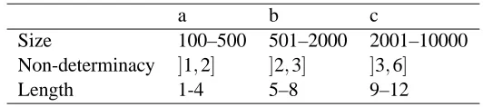
Size 100–500 501–2000 2001–10000 Non-determinacy ]1,2] ]2,3] ]3,6]
Length 1-4 5–8 9–12
Table 2: Discretization of controlled parameters into three categories.
maximal gain can be expected when the first three parameters have large values and the last one is small.
5. Empirical Evaluation
The analysis above gives us some insights into the behaviour of the transformations. In practice, we would like to know the context in which each transformation can be expected to work best. Although theory does not answer this question, it does provide us with the basis on which we can design experiments to provide guidance.
Our empirical evaluation is of two types: (1) controlled experiments using artificial data (Sec-tion 5.1) and (2) uncontrolled experiments using real-world data (Sec(Sec-tion 5.2). All experiments were run on a Linux PC (Pentium III, 850 MHz, 256 MB). We used Aleph 3 running on Yap 4.2.0; coverage lists were enabled throughout.
5.1 Controlled Experiments
The purpose of our controlled experiments is to investigate the influence of parameters on the effi-ciency of the different transformations. We estimate, as a consequence, the set of transformations best suited for each setting of the parameters.
5.1.1 MATERIALS ANDMETHOD
We control the following three parameters: number of examples, length of clauses and non-determinacy. The fourth parameter, complexity of the hardest independent subgoal, is more difficult to control, but can be measured.
We discretize the values of the controlled parameters into three categories: low, medium, high. The thresholds are shown in Table 2. The three categories for three different parameters give rise to 27 combinations. For each combination we generate a corresponding artificial data set and random clauses, then we run the transformations on the clauses and measure the relative performance of each transformation, to determine which one works best for that combination.
5.1.2 THEDATASETS
.
.
.
.
.
.
.
.
.
.
.
.
Figure 4: Relative efficiency of the transformations.
5.1.3 QUERYGENERATION
The clauses generated in this experiment can have two kinds of literals in the body: edge/2 and label/2 literals. The first argument of an edge literal is an input argument; the second argument is then non-determinate as it can take b0 different values. label/2 literals are always added with a constant as second argument and serve as tests (i.e., they may succeed or fail).
The random queries are generated in a levelwise top-down manner, as follows:
C0:={ p(X)← } l := 1
while l<maxclauselength
Cl := n random refinements of random clauses from C increment l
Clauses are then selected at random from the Cl.
5.1.4 RESULTS
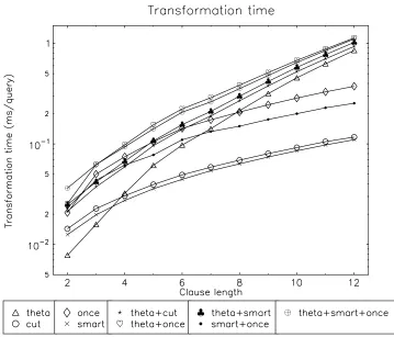
figure), they also give an indication of the actual time they consume. If T(t,l)is the time needed to execute transformation t on a clause of length l, and e is the number of examples, then T(t,l)/e is the time we should at least gain when evaluating a query on a single example for the transformation to be useful.
Figure 5 summarizes results on evaluation times. For each individual clause nondeterminacy was estimated as the average branching factor b=be0/l with b0the branching factor in the graph; e the number of edge literals in the clause, l the length of the clause (since only edge literals have a nondeterminacy of b, label literals are determinate).
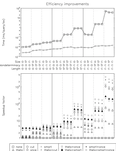
The continuous lines show the actual running times of the slowest and the fastest approach. The graph clearly shows that the longest running times are needed when nondeterminacy as well as clause length are high. The average time for querying one example does not depend much on the size of the data set (which means the total running time is linear in the number of examples). It is also clear that the transformations yield the highest efficiency gain where it counts most, and thus greatly reduce the variance of the timings: execution times for transformed clauses vary over a factor of about 20 instead of a factor of 1000.
Below the absolute measurements, relative speedups are shown; the 1.0 line corresponds to “no transformation”. In almost all cases, all transformations yield a speedup, sometimes a large one. The most complex composed transformation (tθso) consistently yields the greatest speedup.
As all three parameters vary along the same axis in this graph, the effect of each single parameter is a bit obscured. For instance, it is not apparent whether moving from a simple to a more complex setting always increases the speedup. The settings are partially ordered according to complexity. Figure 6 visualizes this partial ordering in a lattice. To keep the lattice simple the effect of data set size is not included; from Figure 5 it is quite clear that data set size does not significantly influence the speedup ratios. The numbers in the nodes of the lattice show the average speedup (averaged over data sets of varying size) for the tθso transformation. It clearly indicates that the speedup indeed increases monotonically with complexity.
5.2 Uncontrolled Experiments
The purpose of the uncontrolled experiments is to examine the performance of the best transforma-tions on particular data sets.
5.2.1 MATERIALS ANDMETHOD
Data here are from real-world problems or benchmarks. With these problems, the procedure in Fig-ure 7 was adopted. In practice, adopting this procedFig-ure is trivial in the sense that for all categories, our experiments on artificial data indicate tθsoas the best transformation.
5.2.2 NOTE ON DATASETS
We used three datasets for these experiments, which have the following properties:
• Bongard (De Raedt and Van Laer, 1995): 1352 examples; nondeterminacy estimate: low
• Carcinogenesis (Srinivasan et al., 1999): 330 examples; nondeterminacy estimate: high
. . . .
. . . .
. . .
. . .
. . .
. . .
. . .
.
Length
Nondeterminacy
Size
Speedup for theta+smart+once
a a 3.80
b a 4.28
a b 6.54
b b 20.6 c a
5.62
a c 21.8
c b 95.8
b c 177
c c 3000
Figure 6: Different settings, partially ordered according to the “is more complex than” relation (excluding the size parameter). In the nodes, speedup factors for tθsoare shown.
1. Assign each problem to one of the 27 categories (obtained previously) 2. Choose the best transformation for the category from controlled experiments 3. Employ transformation and record results
Nondeterminacy estimates are based on the typical use of predicates that occur in the data; for instance, the molecules used in the Carcinogenesis dataset contain on average some 30 atoms; introducing a new atom literal with a free variable identifying the atom thus has a nondeterminacy factor of 30. However, there are also e.g. bond literals with lower nondeterminacy; assuming both occur equally frequently in a clause, it makes sense to estimate nondeterminacy as the geometric mean of all these nondeterminacy factors. Based on this reasoning and on previous experience with these datasets, we estimate nondeterminacy to be low for Bongard, and high for Carcinogenesis and Mutagenesis.
Average clause length is the most difficult parameter to estimate, as it does not follow from the data but depends on the complexity of the target theory. For Carcinogenesis, there is reason to believe that there are no good clauses of small length (Srinivasan et al., 1999), so an estimate of medium to high seems appropriate. For Mutagenesis, previous experience suggests that clause length can be expected to be low. For Bongard underlying theories of arbitrary complexity can be generated; here we varied the maximal clause length from low to high.
The categories are then as follows:
• Bongard: Size=medium, Nondeterminacy=low, Clause length = low-high
• Carcinogenesis: Size=low, Nondeterminacy=high, Clause length = medium-high
• Mutagenesis: Size=low, Nondeterminacy=high, Clause length = low
Our previous analysis predicts tθsoto work best on all three. It also suggests that the speedup factors for query execution that can be obtained with this transformation are: for Bongard, 5 to 20; for Carcinogenesis: 100 to 1000; and for Mutagenesis: 5. Aleph keeps coverage lists for its clauses and the smartcall transformation can be used. However since for other ILP systems it might not be possible to include smartcall in the transformation, it is instructive to examine the results obtained with tθo.
5.2.3 RESULTS
Figures 8, 9 and 10 show the efficiency gains obtained on the Bongard, Carcinogenesis and Muta-genesis data sets. We separate the times consumed by the transformation, the execution of the query in the database, and other computations done by the learner. Note that on the artificial data sets we measured only the speedup of the query execution itself.
We now examine each problem in turn. On the Bongard dataset with small nondeterminacy, only little gain is achieved (Figure 8): even for relatively large clause lengths a speedup factor of about two is achieved, and for small clause lengths the overhead of performing the transformation is not compensated by faster query execution. It is also the case, however, that the overhead imposed by the query transformations is small (less than 5%).
Figure 8: Efficiency improvements obtained on the Bongard data set.
controlled data. Apparently the reduction in SLD-tree size is as expected, but it is not matched by the execution speedup. We have, as yet, been unable to come up with a suitable explanation for this discrepancy.
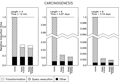
The greatest gain is achieved in the highly nondeterminate Carcinogenesis dataset (Figure 9). When restricting the clause length to 6, Aleph’s total run time was reduced by two orders of mag-nitude, and the query execution time itself by a factor 200. When allowing a maximal clause length of 8, experimentally determining the speedup became impractical. Illustrative examples were still instructive: a certain point in the search space that with transformed clauses took 6 minutes to reach, was only reached after over three days with untransformed clauses. The whole run with transformed clauses took 2.53 hours, and our estimate of the speedup factor is necessarily very approximate. Nevertheless, these results seem consistent with our estimate of 102to 103. The Mu-tagenesis dataset (Figure 10) can be positioned in between. The query execution speedup is here around 4, which is clearly close to what was expected (5).
6. Conclusions
Figure 9: Efficiency improvements obtained on the Carcinogenesis data set.
non-determinate background predicates. We have conducted an empirical study that confirms this and moreover shows that the transformation overhead is sufficiently small so that even on mod-erately sized data sets with simple queries and low non-determinacy, there is no adverse effect of performing the transformations. It is therefore advisable to always use, in practice, the most so-phisticated composition of transformations that is applicable. For systems that refine clauses in a top-down manner and remember the set of examples covered by the parent clause, this is the com-position of the theta, smartcall and once transformations; for other systems the comcom-position of the theta and once transformations is the best option.
The approach adopted in this paper is in the long tradition of source-to-source program trans-formations: changes at the source-level that can improve efficiency without altering correctness (Loveman, 1977). The suggestions here by no means exhaust the transformations of this type. Within ILP, a related approach is described by Blockeel et al. (2000a), where a set of queries is restructured so that they can be executed more efficiently, without changing the individual queries however. The two approaches are obviously complementary, and it would be interesting to see how they can be combined.
Figure 10: Efficiency improvements obtained on the Mutagenesis data set.
then employ a standard execution mechanism, some of the theta-subsumption optimisations might be useful for improving the execution strategy itself.
Finally, we remark that obtaining efficiency gains by means of transformations such as the ones described here is only one side of the story. Efficiency gains are as much to be made by tailoring compilers of logic programs to account for what ILP systems do. The best results regarding effi-ciency may well be obtained by combining both views, i.e., designing Prolog engines in conjunction with ILP algorithms.
Acknowledgments
Appendix A. Program analysis and set sharing for determining (in)dependent calls
Program analysis aims at deriving at compile-time information about the execution of a program. Typically this information could also be given explicitly by the programmer, e.g. a declaration stating that the execution of a predicate grounds it arguments. In (constraint) logic programming re-searchers have been using abstract interpretation (Cousot and Cousot, 1992) as a general framework for program analysis: the concrete execution of a program is mimicked by using descriptions of the concrete substitutions, so-called abstractions. Much research effort has been put into the develop-ment of these abstractions, which have to be safe approximations of their concrete counterparts, but which also have to be precise enough to capture the properties of interest. Again groundness is a very well studied property. Also note that abstract interpretation computes these abstractions at all program points in a program, typically before and after each call such that the abstractions describe all possible concrete substitutions before and after a call.
For this paper we would like to point out the link with the set sharing abstraction (Jacobs and Langen, 1992; Bueno et al., 1994) which has been used to identify possibilities for independent AND-parallelism (Codish et al., 1997) and which can also be used in this context to refine the dependencies between the arguments of the calls. It is beyond the scope of this paper to give a detailed explanation of program analysis topics, but we will show in an informal way how program analysis can help in this context.
Taking into account all variables of the calls for the detection of dependency is a safe abstraction of the execution of the called predicate: execution of the predicate can possibly create dependencies between all the variables in the calls. This approach is compatible with the set sharing abstraction for a call for which no additional information is available and in which all variables are initially free independent variables—the latter is known as a goal-independent analysis. For the call p(X,Y,Z) the set sharing abstraction is the powerset of the set of all its variables{X,Y,Z}, namely{{},{X}, {Y}, {Z}, {X,Y},{X,Z},{Y,Z}, {X,Y,Z}}. A subset in the abstraction describes the possibility that the variables in the subset have in their values variables in common. The above abstraction then describes for example the concrete substitution {X ← f(A,B),Y ← f(A,C),Z ←g(B,A)}. This concrete substitution is not described by the abstraction {{X}, {Y}, {Z},{X,Y},{X,Z}, {Y,Z}} as the sharing of A by{X,Y,Z}is not allowed, nor by the abstraction{{X},{Y},{Z}}as now no shared variables are allowed. The power set safely expresses that we have to assume all possible cases, as we do not know anything about what the call actually does to its free arguments. Reasoning with the largest set of dependent variables is safe as it describes the dependencies we are interested in.
Program analysis allows us to refine the dependency relation between the arguments of calls. A first case is the grounding of variables: as soon as a variable becomes ground it should no longer be considered for dependency determination. In the set sharing abstraction the ground variables are removed from the powerset. This is compatible with the treatment of ground variables. The point here is that program analysis derives this grounding behaviour by computing a more precise abstraction for grounding calls. If the call p(X,Y,Z) grounds all its variables, the abstraction is {}. If only X is grounded, the abstraction is {{Y}, {Z}, {Y,Z}} (which still allows all possible dependencies between Y and Z). Finally, if X and Y are both grounded, the abstraction becomes {{Z}}.
the static version of the once-transformation. For a call p(X,Y,Z) that only can create a dependency between Y and Z, the abstraction is{{X},{Y},{Z},{Y, Z}}. Again, taking all variables of the call would be an overestimation: one can make a distinction between the calls depending on{X}and the ones depending on{Y, Z}. Alternatively, one could for determining dependent calls view p(X,Y,Z) as two independent calls p1(X) and p2(Y,Z) (or similarly as the conjunction p(X, , ), p( ,Y,Z) such that each p/3 call can be part of another set of dependent calls).
Our program analysis based approach could be organised along the following lines. First for all predicates (describing the examples and the background knowledge) a goal-independent set shar-ing analysis is done which can be used to approximate the dependency property of a call (also taking into account the independence of variables). Also for builtins, set sharing can compute an abstraction. Typically, builtins such as comparison impose that the variables are ground, so the set abstraction will be empty. For X = Y, the abstraction is{{X,Y}}. Note this has to be done only once.
Then we consider the calls in a query from left to right together with their dependency approxima-tion (as derived from set sharing abstracapproxima-tions). We will also propagate the groundness informaapproxima-tion from left to right which will remove ground variables from the dependency approximations.5 During this left-to-right traversal we can determine the chains of dependent calls by computing transitive closures on the “grounded” dependency approximations.
Let us consider the following example query wheret(T) is the extension. p(X,Y), q(X,Z), lof(Z), r(Y,T), t(T).
1. In the most general setting, all the calls have as dependency approximation their complete set of variables. Thus they all belong to the same (dependency) chain.
2. Suppose p(X,Y) grounds both X and Y, then we have the following dependency approxima-tion after propagating the groundness: p(X,Y):{}, q(X,Z):{Z}, lof(Z):{Z}, r(Y,T):{T}, t(T): {T}. Thus after the call p(X,Y) there are two chains: q(X,Z), lof(Z) andr(Y,T), t(T). Note that backtracking over values for Z or T is not necessary as soon as a chain has succeeded once.
3. Suppose p(X,Y) grounds neither X nor Y but X and Y remain independent, then the set abstraction is{{X}, {Y}}and we could replace p(X,Y) by the conjunction p(X, ), p( ,Y). The dependency approximation then becomes, p(X, ): {X}, p( ,Y):{Y}, q(X,Z):{{X,Z}}, lof(Z): {{Z}}, r(Y,T): {{Y,T}}, t(T): {T}. We can identify two chains: p(X, ),q(X,Z), lof(Z) andp( ,Y),r(Y,T), t(T).
4. Suppose p(X,Y) grounds only one variable, let us assume X. Then we have two chains:
q(X,Z), lof(Z) andp( ,Y),r(Y,T), t(T).
Appendix B. Generation of Artificial Data Sets
Figure 11 describes the method used for generating artificial data sets and clauses for our first set of experiments. As explained in Section 5.1.2, the data sets are directed graphs containing a number of nodes s and for each node b0outgoing edges.
for each length l from{1−4,5−8,9−12}
Q
=sample 30 clauses of length lfor each branching factor b0from{1−3,4−6,7−9}
for each size s from{100−500,501−2000, 2001−10000} D=generate problem(s, b0)
for each clause q∈
Q
for each transformation t∈
T
q0=transform(t, q) T =time(q0, D)
b=be0/l, with e the number of edges in q compute average time(s,b0,l,T )
Figure 11: Experimental method for controlled experiments
The algorithm generates values for three parameters: the clause length l, the branching factor b0 (i.e. the number of outgoing edges) and the size s. Each parameter can take values from three intervals: low, medium and high. The for-loops are iterated three times, each time selecting a random value from one of the intervals.
A set of clauses
Q
is generated for each length l. Likewise a random graph dataset D is generated based on the values of s and b0. The two most inner loops apply every transformation to each of the clauses inQ
and measure the execution time of the transformed clauses.The parameter b=be0/l, with e the number of edge literals, is an estimate for the nondeterminacy of the clause q. This correction on b0is necessary because only edge literals have a nondeterminacy of b0, label literals are determinate. A side effect of this transformation is that the parameter b has continuous values. These continues values are discretized into three intervals as shown in Table 2.
Average execution times are computed for each of the 27 combinations of s, b and l. To obtain reliable averages, we repeat the entire experiment 100 times. The average times and the correspond-ing speedups are plotted in Figure 5.
References
H. Blockeel. Top-down induction of first order logical decision trees. PhD the-sis, Department of Computer Science, Katholieke Universiteit Leuven, 1998. URL
http://www.cs.kuleuven.ac.be/˜ml/PS/blockeel98:phd.ps.gz.
H. Blockeel, B. Demoen, L. Dehaspe, G. Janssens, J. Ramon, and H. Vandecasteele. Executing query packs in ILP. In J. Cussens and A. Frisch, editors, Proceedings of the 10th International Conference in Inductive Logic Programming, volume 1866 of Lecture Notes in Artificial Intelli-gence, pages 60–77, London, UK, July 2000a. Springer.
I. Bratko and M. Grobelnik. Inductive learning applied to program construction and verification. In Stephen Muggleton, editor, Proceedings of the Third International Workshop on Inductive Logic Programming, pages 279–292. Joˇzef Stefan Institute, 1993.
F. Bueno, M. Garc´ıa de la Banda, and M. Hermenegildo. Effectiveness of global analysis in strict independence-based automatic program parallelization. In International Symposium on Logic Programming, pages 320–337. MIT Press, 1994.
M. Codish, M. Bruynooghe, M. Garc´ıa de la Banda, and M. Hermenegildo. Exploiting goal inde-pendence in the analysis of logic programs. Journal of Logic Programming, 32(3), 1997.
P. Cousot and R. Cousot. Abstract interpretation and application to logic programs. Journal of Logic Programming, 13(2-3):103–179, 1992.
J. Cussens. Part-of-speech tagging using Progol. In Nada Lavraˇc and Saˇso Dˇzeroski, editors, Proceedings of the Seventh International Workshop on Inductive Logic Programming, Lecture Notes in Artificial Intelligence, pages 93–108. Springer-Verlag, 1997.
L. De Raedt and W. Van Laer. Inductive constraint logic. In Klaus P. Jantke, Takeshi Shinohara, and Thomas Zeugmann, editors, Proceedings of the Sixth International Workshop on Algorithmic Learning Theory, volume 997 of Lecture Notes in Artificial Intelligence, pages 80–94. Springer-Verlag, 1995.
L. Dehaspe and H. Toivonen. Discovery of frequent datalog patterns. Data Mining and Knowledge Discovery, 3(1):7–36, 1999.
B. Dolˇsak and S. Muggleton. The application of Inductive Logic Programming to finite element mesh design. In S. Muggleton, editor, Inductive Logic Programming, pages 453–472. Academic Press, 1992.
S. Dˇzeroski, L. Dehaspe, B. Ruck, and W. Walley. Classification of river water quality data using machine learning. In Proceedings of the 5th International Conference on the Development and Application of Computer Techniques to Environmental Studies, 1994.
W. Emde and D. Wettschereck. Relational instance-based learning. In L. Saitta, editor, Proceed-ings of the Thirteenth International Conference on Machine Learning, pages 122–130. Morgan Kaufmann, 1996.
C. Feng. Inducing temporal fault dignostic rules from a qualitative model. In S. Muggleton, editor, Inductive Logic Programming. Academic Press, London, 1992.
D. Jacobs and A. Langen. Static analysis of logic programmings for independent and-parallelism. Journal of Logic Programming, 13:291–314, 1992.
R.D. King, S. Muggleton, R.A. Lewis, and M.J.E. Sternberg. Drug design by machine learning: the use of inductive logic programming to model the structure-activity relationships of trimethoprim analogues binding to dihydrofolate reductase. Proceedings of the National Academy of Sciences, 89(23), 1992.
R.D. King, S. Muggleton, A. Srinivasan, and M.J.E. Sternberg. Structure-activity relationships de-rived by machine learning: The use of atoms and their bond connectivities to predict mutagenicity by inductive logic programming. Proceedings of the National Academy of Sciences, 93:438–442, 1996.
Stefan Kramer. Structural regression trees. In Proceedings of the Thirteenth National Conference on Artificial Intelligence, pages 812–819, Cambridge/Menlo Park, 1996. AAAI Press/MIT Press.
J.W. Lloyd. Foundations of Logic Programming. Springer-Verlag, 2nd edition, 1987.
D. B. Loveman. Program improvement by source-to-source transformation. Journal of the Associ-ation for Computing Machinery, 24(1):121–145, 1977.
E. McCreath. Induction in First Order Logic from Noisy Training Examples and Fixed Example Set Sizes. PhD thesis, University of New South Wales, 1999.
S. Muggleton. Inductive Logic Programming: derivations, successes and shortcomings. SIGART Bulletin, 5(1):5–11, 1994.
S. Muggleton. Inverse entailment and Progol. New Generation Computing, Special issue on Induc-tive Logic Programming, 13(3-4):245–286, 1995.
S. Muggleton and C. Feng. Efficient induction of logic programs. In Proceedings of the First Conference on Algorithmic Learning Theory, pages 368–381. Ohmsma, Tokyo, Japan, 1990.
S. Muggleton, R.D. King, and M.J.E. Sternberg. Protein secondary structure prediction using logic. Protein Engineering, 7:647–657, 1992.
C. N´edellec, H. Ad´e, F. Bergadano, and B. Tausend. Declarative bias in ILP. In L. De Raedt, editor, Advances in Inductive Logic Programming, volume 32 of Frontiers in Artificial Intelligence and Applications, pages 82–103. IOS Press, 1996.
S.-H. Nienhuys-Cheng and R. De Wolf. Foundations of Inductive Logic Programming, volume 1228 of Lecture Notes in Computer Science and Lecture Notes in Artificial Intelligence. Springer-Verlag, New York, NY, USA, 1997.
J.R. Quinlan. Learning logical definitions from relations. Machine Learning, 5:239–266, 1990.
V. Santos Costa, A. Srinivasan, and R. Camacho. A note on two simple transformations for im-proving the efficiency of an ILP system. In J. Cussens and A. Frisch, editors, Proceedings of the Tenth International Conference on Inductive Logic Programming, volume 1866 of Lecture Notes in Artificial Intelligence, pages 225–242. Springer-Verlag, 2000.
M. Sebag and C. Rouveirol. Tractable induction and classification in first-order logic via stochastic matching. In Proceedings of the 15th International Joint Conference on Artificial Intelligence, pages 888–893. Morgan Kaufmann, 1997.
A. Srinivasan. A study of two sampling methods for analysing large datasets with ILP. Data Mining and Knowledge Discovery, 3(1):95–123, 1999.
A. Srinivasan, R.D. King, and D.W. Bristol. An assessment of ILP-assisted models for toxicology and the PTE-3 experiment. In Proceedings of the Ninth International Workshop on Inductive Logic Programming, volume 1634 of Lecture Notes in Artificial Intelligence, pages 291–302. Springer-Verlag, 1999.
A. Srinivasan, S.H. Muggleton, M.J.E. Sternberg, and R.D. King. Theories for mutagenicity: A study in first-order and feature-based induction. Artificial Intelligence, 85(1,2):277–299, 1996.
Ashwin Srinivasan. The Aleph Manual. University of Oxford, 2001.
Patrick R. J. van der Laag and Shan-Hwei Nienhuys-Cheng. Completeness and properness of refine-ment operators in inductive logic programming. Journal of Logic Programming, 34(3):201–225, 1998.