Inconsistency of Pitman–Yor Process Mixtures
for the Number of Components
Jeffrey W. Miller jeffrey miller@brown.edu
Matthew T. Harrison matthew harrison@brown.edu
Division of Applied Mathematics Brown University
Providence, RI 02912, USA
Editor:Yee Whye Teh
Abstract
In many applications, a finite mixture is a natural model, but it can be difficult to choose an appropriate number of components. To circumvent this choice, investigators are increas-ingly turning to Dirichlet process mixtures (DPMs), and Pitman–Yor process mixtures (PYMs), more generally. While these models may be well-suited for Bayesian density esti-mation, many investigators are using them for inferences about the number of components, by considering the posterior on the number of components represented in the observed data. We show that this posterior is not consistent—that is, on data from a finite mixture, it does not concentrate at the true number of components. This result applies to a large class of nonparametric mixtures, including DPMs and PYMs, over a wide variety of families of component distributions, including essentially all discrete families, as well as continuous exponential families satisfying mild regularity conditions (such as multivariate Gaussians).
Keywords: consistency, Dirichlet process mixture, number of components, finite mixture, Bayesian nonparametrics
1. Introduction
We begin with a motivating example. In population genetics, determining the “population structure” is an important step in the analysis of sampled data. To illustrate, consider the impala, a species of antelope in southern Africa. Impalas are divided into two subspecies: the common impala occupying much of the eastern half of the region, and the black-faced impala inhabiting a small area in the west. While common impalas are abundant, the number of black-faced impalas has been decimated by drought, poaching, and declining resources due to human and livestock expansion. To assist conservation efforts, Lorenzen et al. (2006) collected samples from 216 impalas, and analyzed the genetic variation between/within the two subspecies.
A key part of their analysis consisted of inferring the population structure—that is, par-titioning the data into distinct populations, and in particular, determining how many such populations there are. To infer the impala population structure, Lorenzen et al. employed a widely-used tool calledStructure(Pritchard et al., 2000) which, in the simplest version,
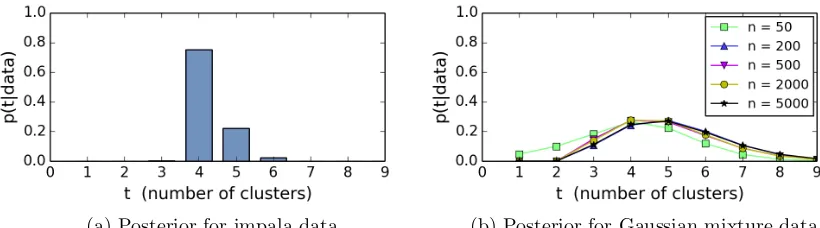
(a) Posterior for impala data (b) Posterior for Gaussian mixture data
Figure 1: Estimated DPM posterior distributions of the number of clusters, with concentration parameter 1: (a) For the impala data of Lorenzen et al. (n= 216 data points); we use the same base measure as Huelsenbeck and Andolfatto, and our empirical results, shown here, agree with theirs. (b) For data from the three-component univariate Gaussian mixtureP3
i=1πiN(x|µi, σ2i) withπ= (0.45,0.3,0.25),µ= (4,6,8), andσ= (1,0.2,0.6); we use a base measure with the same parameters as Richardson and Green (1997); each plot is the average over 10 independently-drawn data sets. For both (a) and (b), estimates were made via Gibbs sampling (MacEachern, 1994; Neal, 2000), with 105 burn-in sweeps
and 2×10⁵ sample sweeps.
to a distinct population. Structure uses an ad hoc method to choose the number of
components, but this comes with no guarantees.
Seeking a more principled approach, Pella and Masuda (2006) proposed using a Dirich-let process mixture (DPM). Now, in a DPM, the number of components is infinite with probability 1, and thus the posterior on the number of components is always, trivially, a point mass at infinity. Consequently, Pella and Masuda instead employed the posterior on the number of clusters (that is, the number of components used in generating the data observed so far) for inferences about the number of components. (The terms “component” and “cluster” are often used interchangeably, but we make the following crucial distinction: a component is part of a mixture distribution, while a cluster is the set of indices of data points coming from a given component.) This DPM approach was implemented in a soft-ware tool calledStructurama(Huelsenbeck and Andolfatto, 2007), and demonstrated on
the impala data of Lorenzen et al.; see Figure 1(a).
Structurama has gained acceptance within the population genetics community, and
has been used in studies of a variety of organisms, from apples and avocados, to sardines and geckos (Richards et al., 2009; Chen et al., 2009; Gonzalez and Zardoya, 2007; Leach´e and Fujita, 2010). Studies such as these can carry significant weight, since they may be used by officials to make informed policy decisions regarding agriculture, conservation, and public health.
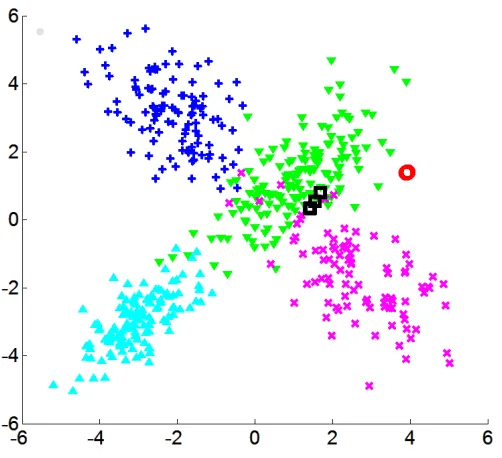
Figure 2: A typical partition sampled from the posterior of a Dirichlet process mixture of bivariate Gaussians, on simulated data from a four-component mixture. Different clusters have different marker shapes (+,×,O,M,
◦
,2) and different colors. Note the tiny “extra” clusters (◦
and2), in addition to the four dominant clusters.of clusters—not just the density—on the assumption that this is informative about the number of components. Further examples include gene expression profiling (Medvedovic and Sivaganesan, 2002), haplotype inference (Xing et al., 2006), survival analysis (Argiento et al., 2009), econometrics (Otranto and Gallo, 2002), and evaluation of inference algo-rithms (Fearnhead, 2004). Of course, if the data-generating process is well-modeled by a DPM, then it is sensible to use this posterior for inference about the number of components represented so far in the data—but that does not seem to be the perspective of these in-vestigators, since they measure performance on simulated data coming from finitely many components or populations.
Therefore, it is important to understand the properties of this procedure. Simulation results give some cause for concern; for instance, Figure 1(b) displays results on data from a mixture of univariate Gaussians with three components. The posterior on the number of clusters does not appear to be concentrating as the number of data points n increases. Empirically, it seems that this is because partitions sampled from the posterior often have tiny, transient “extra” clusters (as has been noted before, see Section 1.2); for instance, see Figure 2, showing a typical posterior sample on data from a four-component mixture of bivariate Gaussians. This raises a fundamental question that has not been addressed in the literature: With enough data, will this posterior eventually concentrate at the true number of components? In other words, is it consistent?
posterior—it may be that the likelihood is strong enough to overcome this prior tendency. Of course, in a typical Bayesian setting, the prior is fixed, and asnincreases the likelihood overwhelms it. In the present situation, though, both the prior (on the number of clusters) and the likelihood (given the number of clusters) are changing with n, and the resulting behavior of the posterior is far from obvious.
1.1 Overview of Results
In this manuscript, we prove that under fairly general conditions, when using a Dirichlet process mixture, the posterior on the number of clusters will not concentrate at any finite value, and therefore will not be consistent for the number of components in a finite mixture. In fact, our results apply to a large class of nonparametric mixtures including DPMs, and Pitman–Yor process mixtures (PYMs) more generally, over a wide variety of families of component distributions.
Before treating our general results and their prerequisite technicalities, we would like to highlight a few interesting special cases that can be succinctly stated. The terminology and notation used below will be made precise in later sections. To reiterate, our results are considerably more general than the following corollary, which is simply presented for the reader’s convenience.
Corollary 1 Consider a Pitman–Yor process mixture with component distributions from one of the following families:
(a) Normal(µ,Σ) (multivariate Gaussian),
(b) Exponential(θ),
(c) Gamma(a, b),
(d) Log-Normal(µ, σ2), or
(e) Weibull(a, b) with fixed shape a >0,
along with a base measure that is a conjugate prior of the form in Section 5.2, or
(f ) any discrete family{Pθ} such thatTθ{x:Pθ(x)>0} 6=∅(e.g., Poisson, Geometric, Negative Binomial, Binomial, Multinomial, etc.),
along with any continuous base measure. Consider any t∈ {1,2, . . .}, except for t=N in the case of a Pitman–Yor process with parameters σ <0 and ϑ=N|σ|. If X1, X2, . . . are i.i.d. from a mixture withtcomponents from the family used in the model, then the posterior on the number of clusters Tn is not consistent fort, and in fact,
lim sup n→∞
p(Tn=t|X1:n)<1
This is implied by Theorems 6, 7, and 11. These more general theorems apply to a broad class of partition distributions, handling Pitman–Yor processes as a special case, and they apply to many other families of component distributions: Theorem 11 covers a large class of exponential families, and Theorem 7 covers families satisfying a certain boundedness condition on the densities (including any case in which the model and data distributions have one or more point masses in common, as well as many location–scale families with scale bounded away from zero). Dirichlet processes are subsumed as a further special case, being Pitman–Yor processes with parameters σ = 0 and ϑ > 0. Also, the assumption of i.i.d. data from a finite mixture is much stronger than what is required by these results.
For PYMs withσ∈[0,1) (including DPMs), our results show thatp(Tn=t|X1:n) does not concentrate at any finite value, however, we have not been able to determine the precise limiting behavior of this posterior; the two most plausible outcomes are that it diverges, or stabilizes at some limiting distribution.
Regarding the exception of t=N when σ <0 in Corollary 1: posterior consistency at
t=N is possible, however, this could only occur if the chosen parameterN just happens to be equal to the actual number of components, t. On the other hand, consistency at any t
can (in principle) be obtained by putting a prior onN; see Section 1.2.1 below. In a similar vein, some investigators place a prior on the concentration parameterϑin a DPM, or allow
ϑto depend onn; we conjecture that inconsistency can still occur in these cases, but in this paper, we examine only the case of fixed σ and ϑ.
Truncated stick-breaking processes (Ishwaran and James, 2001) are sometimes used to approximate nonparametric models. In a very limited case—see Section 2.1—our results show that on data from a one-component mixture, such a process truncated at two com-ponents will be inconsistent for the number of comcom-ponents. It seems likely that this will extend to truncations at any number of components.
1.2 Discussion / Related Work
We would like to emphasize that this inconsistency should not be viewed as a deficiency of DPMs and PYMs, but is simply due to a misapplication of them. As flexible priors on densities, DPMs are superb, and there are strong results showing that in many cases the posterior on the density converges in L1 to the true density at the minimax-optimal
rate, up to logarithmic factors (Ghosal et al., 1999; Ghosal and Van der Vaart, 2001; Lijoi et al., 2005; Tokdar, 2006; Ghosh and Ghosal, 2006; Tang and Ghosal, 2007; Ghosal and Van der Vaart, 2007; Walker et al., 2007; James, 2008; Wu and Ghosal, 2010; Bhattacharya and Dunson, 2010; Khazaei et al., 2012; Scricciolo, 2012; Pati et al., 2013); for a general overview, see Ghosal (2010).
Existing work on posterior consistency of nonparametric mixtures has been primarily focused on the density estimation problem (as mentioned above), although recently, Nguyen (2013) has shown that the DPM posterior on the mixing distribution converges in the Wasserstein metric to the true mixing distribution. These existing results do not necessarily imply consistency for the number of components, since any mixture can be approximated arbitrarily well in these metrics by another mixture with a larger number of components (for instance, by making the weights of the extra components infinitesimally small). There seems to be no prior work on consistency of DPMs or PYMs for the number of components in a finite mixture (aside from Miller and Harrison, 2013, in which we discuss the very special case of a DPM on data from a univariate Gaussian “mixture” with one component of known variance).
In the context of “species sampling”, several authors have studied the Pitman–Yor process posterior (Pitman, 1996; Hansen and Pitman, 2000; James, 2008; Jang et al., 2010; Lijoi et al., 2007, 2008), and interestingly, James (2008) and Jang et al. (2010) have shown that on data from a continuous distribution, the posterior of a Pitman–Yor process with
σ >0 is inconsistent in the sense that it does not converge weakly to the true distribution. (In contrast, the Dirichlet process is consistent in this sense.) However, this is very different from our situation—in a species sampling model, the observed data is drawn directly from a discrete measure with a Pitman–Yor process prior, while in a PYM model, the observed data is drawn from a mixture with such a measure as the mixing distribution.
Rousseau and Mengersen (2011) proved an interesting result on “overfitted” mixtures, in which data from a finite mixture is modeled by a finite mixture with too many components. In cases where this approximates a DPM, their result implies that the posterior weight of the extra components goes to zero. In a rough sense, this is complementary to our results, which involve showing that there are always some nonempty (but perhaps small) extra clusters.
Empirically, many investigators have noticed that the DPM posterior tends to overes-timate the number of components (e.g., West et al., 1994; Ji et al., 2010; Argiento et al., 2009; Lartillot and Philippe, 2004; Onogi et al., 2011, and others), and such observations are consistent with our theoretical results. This overestimation seems to occur because there are typically a few tiny “extra” clusters, and among researchers using DPMs for clustering, this is an annoyance that is sometimes dealt with by pruning such clusters—that is, by removing them before calculating statistics such as the number of clusters (e.g., West et al., 1994; Fox et al., 2007). It may be possible to obtain consistent estimators in this way, but this remains an open question; Rousseau and Mengersen’s (2011) results may be applicable here. Other possibilities are using a maximum a posteriori (MAP) partition or posterior “mean” partition (Dahl, 2006; Huelsenbeck and Andolfatto, 2007; Onogi et al., 2011) to estimate the number of components; again, the consistency of such approaches remains an open question to our knowledge.
1.2.1 Estimating the Number of Components
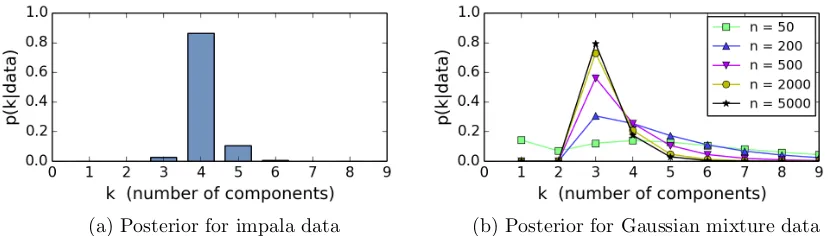
(a) Posterior for impala data (b) Posterior for Gaussian mixture data
Figure 3: Estimated posterior distributions of the number of components for variable-dimension mixture models applied to the same data sets as in Figure 1. The same priors on com-ponent parameters (base measures) were used as in the DPM models.
2000; Nobile, 1994; Leroux, 1992; Ishwaran et al., 2001; James et al., 2001; Henna, 2005; Woo and Sriram, 2006, 2007).
From the Bayesian perspective, perhaps the most natural approach is simply to take a finite mixture model and put a prior on the number of components. For instance, draw the number of components k from a prior which is positive on all positive integers (so there is no a priori upper bound), draw mixture weights (π1, . . . , πk) from, say, a k-dimensional Dirichlet distribution, draw component parametersθ1, . . . , θk, and draw the dataX1, . . . , Xn from the resulting mixture. (Interestingly, it turns out that putting a prior on N in a PYM with σ < 0 and ϑ = N|σ| is a special case of this; see Gnedin and Pitman, 2006.) Such variable-dimension mixture models have been widely used (Nobile, 1994; Phillips and Smith, 1996; Richardson and Green, 1997; Stephens, 2000; Green and Richardson, 2001; Nobile and Fearnside, 2007), and for density estimation, they have been shown to have posterior rates of concentration similar to Dirichlet process mixtures (Kruijer, 2008; Kruijer et al., 2010). Under the (strong) assumption that the family of component distributions is correctly specified, it has been proven that such models exhibit posterior consistency for the number of components (as well as for the mixing measure and the density) under very general conditions (Nobile, 1994).
Figure 3 shows the posterior on the number of components k for variable-dimension mixture models applied to the same impala data and Gaussian mixture data as in Figure 1. In Figure 3(b), the posterior onkseems to be concentrating at the true number of compo-nents (as expected, due to Nobile, 1994), while in Figure 1(b) the DPM posterior does not appear to be concentrating (as expected, due to our results). There is enough information in the data to make the posterior concentrate at the true value; the problem with the DPM posterior is not that estimating the number of components is inherently difficult, but that the DPM posterior is simply the wrong tool for this job.
since any sufficiently regular density can be approximated arbitrarily well by a mixture of Gaussians, if the data distribution is close to but not exactly a finite mixture of Gaussians, a Gaussian mixture model will introduce more and more components as the amount of data increases. It seems that in order to obtain reliable assessments of heterogeneity using mixture models, one needs to carefully consider the effects of potential misspecification. Steps toward addressing this robustness issue have been taken by Woo and Sriram (2006, 2007).
1.3 Idea of the Proof
Roughly speaking, the reason why the posterior on the number of clusters does not con-centrate for PYMs withσ ∈[0,1) (the σ <0 case is somewhat different) is that under the prior, the partition distribution strongly prefers that some of the clusters be very small, and the likelihood is not significantly decreased by splitting off such small clusters. Handling the likelihood—in a general setting—is the challenging part of the proof.
The proof involves showing that p(Tn = t+ 1 | X1:n) is at least the same order of magnitude (asymptotically with respect ton) asp(Tn=t|X1:n). To get the basic idea of why this occurs, write
p(Tn=t|X1:n) =
p(X1:n, Tn=t)
p(X1:n)
= 1
p(X1:n) X
A∈At(n)
p(X1:n|A)p(A), (1)
where the sum is over all partitionsA of{1, . . . , n} intotparts.
Now, given somet-part partitionA, supposeBis a (t+1)-part partition obtained fromA
by splitting off a single elementjto be in its own cluster. For Pitman–Yor processes,p(B) is at least the same order of magnitude asp(A)/n. In Section 3, this property is encapsulated in Condition 3, which is simple to check for any closed-form partition distribution.
Similarly, it turns out that typically, for a non-negligible fraction of the elements j, the likelihoodp(X1:n|B) is at least the same order of magnitude asp(X1:n|A); in Section 3, this is made precise in Condition 4. This is trivial in discrete cases (see Section 4), and often is easy to show in any particular continuous case, but establishing this condition in a general setting requires some work, and it is this that occupies the bulk of the proof (Section 8 and the appendices).
When both of these conditions are satisfied, we show that in the expression for p(Tn=
t | X1:n) in Equation 1, for each term p(X1:n|A)p(A) there are on the order of n terms
p(X1:n|B)p(B) in the corresponding expression for p(Tn=t+ 1|X1:n) that collectively are at least the same order of magnitude as p(X1:n|A)p(A).
1.4 Organization of the Paper
the theorem to cases in which the mixture is over an exponential family satisfying some regularity conditions. The rest of the paper contains proofs of the results described in the previous sections: Section 7 contains the proof of the general theorem and its application to discrete or bounded cases, Section 8 contains the proof of the application to exponential families, and the appendices contain a number of supporting results for the exponential family case.
2. Model Distribution
Our analysis involves two probability distributions: one which is defined by the model, and another which gives rise to the data. In this section, we describe the model distribution.
Building upon the Dirichlet process (Ferguson, 1973; Blackwell and MacQueen, 1973; Antoniak, 1974), Dirichlet process mixtures were first studied by Antoniak (1974), Berry and Christensen (1979), Ferguson (1983), and Lo (1984), and were later made practical through the efforts of a number of authors (Escobar, 1988; MacEachern, 1994; Escobar and West, 1995; West, 1992; West et al., 1994; Neal, 1992; Liu, 1994; Bush and MacEachern, 1996; MacEachern and M¨uller, 1998; MacEachern, 1998; Escobar and West, 1998; MacEachern, 1999; Neal, 2000). Pitman–Yor process mixtures (Ishwaran and James, 2001, 2003) are a generalization of DPMs based on the Pitman–Yor process (Perman et al., 1992; Pitman and Yor, 1997), also known as the two-parameter Poisson–Dirichlet process. We consider a general class of partition-based mixture models that includes DPMs and PYMs.
2.1 Partition Distribution
We will use p(·) to denote probabilities and probability densities under the model. Our model specification begins with a distribution on partitions, or more precisely, on ordered
partitions. Givenn∈ {1,2, . . .} and t∈ {1, . . . , n}, let At(n) denote the set of all ordered partitionsA= (A1, . . . , At) of{1, . . . , n}intotnonempty sets (or “parts”). In other words,
At(n) = n
(A1, . . . , At) :A1, . . . , Atare disjoint, t [
i=1
Ai={1, . . . , n}, |Ai| ≥1 ∀i o
.
For eachn∈ {1,2, . . .}, consider a probability mass function (p.m.f.) p(A) on Sn
t=1At(n).
This induces a distribution ontin the natural way, viap(t|A) =I(A∈ At(n)). (Through-out, we use I to denote the indicator function: I(E) is 1 if E is true, and 0 otherwise.) It follows thatp(A) =p(A, t) when A∈ At(n).
For example, the partition distribution for the Dirichlet process is
p(A) = ϑ t
ϑn↑1 t!
t Y
i=1
(|Ai| −1)! (2)
forA∈ At(n), whereϑ >0 andxn↑δ =x(x+δ)(x+ 2δ)· · ·(x+ (n−1)δ), withx0↑δ= 1 by convention. Thet! in the denominator appears since we are working with ordered partitions. More generally, the partition distribution for the Pitman–Yor process is
p(A) = (ϑ+σ)t−1↑σ (ϑ+ 1)n−1↑1 t!
t Y
i=1
(1−σ)|Ai|−1↑1 (3)
forA ∈ At(n), where eitherσ ∈[0,1) and ϑ∈(−σ,∞), or σ ∈(−∞,0) and ϑ=N|σ|for someN ∈ {1,2, . . .}. Whenσ = 0, this reduces to the partition distribution of the Dirichlet process. When σ < 0 and ϑ= N|σ|, it is the partition distribution obtained by drawing
q = (q1, . . . , qN) from a symmetric N-dimensional Dirichlet with parameters |σ|, . . . ,|σ|, sampling assignments Z1, . . . , Zni.i.d. from q, and removing any empty parts (Gnedin and Pitman, 2006). Thus, in this latter case, tis always in {1, . . . , N}.
Stick-breaking processes truncated atN components are sometimes used to approximate nonparametric models (Ishwaran and James, 2001). This approach gives rise to a partition distribution as follows: letVi∼Beta(ai, bi) independently fori= 1, . . . , N−1, andVN = 1, set qi =ViQj<i(1−Vj) for i= 1, . . . , N, sample assignmentsZ1, . . . , Zn i.i.d. fromq, and remove any empty parts. In general, it seems that this partition distribution takes a slightly complicated form, however, in the very special case when N = 2 and a1 =b1, it is simply
a Pitman–Yor process withσ =−a1 =−b1 and ϑ= 2|σ|. 2.2 Partition-based Mixture Model
Consider the hierarchical model
p(A, t) =p(A)
p(θ1:t|A, t) = t Y
i=1
π(θi) (4)
p(x1:n|θ1:t, A, t) = t Y
i=1
Y
j∈Ai
pθi(xj)
whereπis a prior density on component parametersθ∈Θ⊂Rkfor somek, and{p
θ :θ∈Θ} is a parameterized family of densities on x∈ X ⊂Rd for somed. Here,x
1:n= (x1, . . . , xn) with xi ∈ X, θ1:t = (θ1, . . . , θt) with θi ∈ Θ, and A ∈ At(n). Assume that π is a density with respect to Lebesgue measure, and that {pθ : θ ∈ Θ} are densities with respect to some sigma-finite Borel measure λ on X, such that (θ, x) 7→ pθ(x) is measurable. (The distribution of x underpθ(x) may be discrete, continuous, or neither, depending onλ.)
For x1, . . . , xn∈ X and J ⊂ {1, . . . , n}, define thesingle-cluster marginal,
m(xJ) = Z
Θ
Y
j∈J
pθ(xj)
wherexJ = (xj :j∈J), and assume m(xJ)<∞. By convention,m(xJ) = 1 when J =∅.
Note thatm(xJ) is a density with respect to the product measureλ` onX`, where`=|J|, and thatm(xJ) can (and often will) be positive outside the support ofλ`.
Definition 2 We refer to such a hierarchical model as a partition-based mixture model.
In particular, it is aDirichlet process mixture model whenp(A) is as in Equation 2, or more generally, aPitman–Yor process mixture model when p(A) is as in Equation 3.
The prior on the number of clusters under such a model is p(Tn=t) =PA∈At(n)p(A). We useTn, rather thanT, to denote the random variable representing the number of clusters, as a reminder that its distribution depends onn.
Since we are concerned with the posteriorp(Tn=t|x1:n) on the number of clusters, we will be especially interested in the marginal density of (x1:n, t), given by p(x1:n, Tn =t) = P
A∈At(n)p(x1:n, A). Observe that
p(x1:n, A) =p(A) t Y
i=1
Z Y
j∈Ai
pθi(xj)
π(θi)dθi =p(A) t Y
i=1
m(xAi). (6)
For definiteness, we employ the usual version of the posterior of Tn,
p(Tn=t|x1:n) =
p(x1:n, Tn=t)
p(x1:n)
= P∞p(x1:n, Tn=t) t0=1p(x1:n, Tn=t0)
whenever the denominator is nonzero, and p(Tn = t | x1:n) = 0 otherwise (for notational convenience).
3. General Theorem
The essential ingredients in the main theorem are Conditions 3 and 4 below. ForA∈ At(n), define RA = Si:|Ai|≥2Ai, and for j ∈ RA, define B(A, j) to be the element B of At+1(n)
such that Bi =Airj for i= 1, . . . , t, and Bt+1 = {j} (that is, remove j from whatever
part it belongs to, and make {j} the (t+ 1)th part). Let ZA = {B(A, j) : j ∈ RA}. For
n > t≥1, define
cn(t) = 1
nAmax∈At(n) max B∈ZA
p(A)
p(B), (7)
with the convention that 0/0 = 0 and y/0 =∞ fory >0.
Condition 3 Assume lim supn→∞cn(t)<∞, given some particular t∈ {1,2, . . .}.
For Pitman–Yor processes, Condition 3 holds for all relevant values of t; see Proposition 5 below. Now, givenn≥t≥1,x1, . . . , xn∈ X, andc∈[0,∞), define
ϕt(x1:n, c) = min A∈At(n)
1
n|SA(x1:n, c)|
Condition 4 Given a sequence of random variables X1, X2, . . . ∈ X, and t ∈ {1,2, . . .}, assume
sup c∈[0,∞)
lim inf
n→∞ ϕt(X1:n, c)>0 with probability1.
Note that Condition 3 involves only the partition distributions, while Condition 4 in-volves only the data distribution and the single-cluster marginals.
Proposition 5 Consider a Pitman–Yor process. If σ ∈[0,1) and ϑ∈(−σ,∞) then Con-dition 3 holds for any t∈ {1,2, . . .}. If σ ∈ (−∞,0) and ϑ=N|σ|, then it holds for any t∈ {1,2, . . .} except N.
Proof See Section 7.
Theorem 6 LetX1, X2, . . .∈ X be a sequence of random variables (not necessarily i.i.d.). Consider a partition-based mixture model. For any t ∈ {1,2, . . .}, if Conditions 3 and 4 hold, then
lim sup
n→∞ p(Tn=t
|X1:n)<1 with probability 1.
If, further, the sequence X1, X2, . . . is i.i.d. from a mixture with t components, then with probability 1, the posterior of Tn (under the model) is not consistent fort.
Proof See Section 7.
4. Application to Discrete or Bounded Cases
By Theorem 6, the following result implies inconsistency in a large class of PYM models, including essentially all discrete cases (or more generally anything with at least one point mass) and a number of continuous cases as well.
Theorem 7 LetX1, X2, . . .∈ X be a sequence of random variables (not necessarily i.i.d.). If there exists U ⊂ X such that
(1) lim inf n→∞
1
n
n X
j=1
I(Xj ∈U)>0 with probability 1, and
(2) supnpθ(x)
m(x) :x∈U, θ∈Θ
o
<∞ (where 0/0 = 0, y/0 =∞ for y >0),
then Condition 4 holds for allt∈ {1,2, . . .}.
Proof See Section 7.
(i) Finite sample space. SupposeX is a finite set,λis counting measure, andm(x)>0 for all x ∈ X. Then choosing U = X, Conditions 7(1) and 7(2) of Theorem 7 are trivially satisfied, regardless of the distribution of X1, X2, . . .. (Note that when λ is
counting measure, pθ(x) and m(x) are p.m.f.s on X.) It is often easy to check that
m(x) > 0 by using the fact that this is true whenever {θ ∈ Θ : pθ(x) > 0} has nonzero probability under π. This case covers, for instance, Multinomials (including Binomials), and the population genetics model from Section 1.
We should mention a subtle point here: when X is finite, mixture identifiability might only hold up to a certain maximum number of components (e.g., Teicher, 1963, Proposition 4, showed this for Binomials), making consistency impossible in general— however, consistency might still be possible within that identifiable range. Regardless, our result shows that PYMs are not consistent anyway.
Now, suppose P is a probability measure on X, and X1, X2, . . . iid
∼ P. Let us abuse notation and writeP(x) =P({x}) andλ(x) =λ({x}) for x∈ X.
(ii) One or more point masses in common. If there existsx0∈ X such thatP(x0)>
0, λ(x0) >0, and m(x0)> 0, then it is easy to verify that Conditions 7(1) and 7(2)
are satisfied with U = {x0}. (Note that λ(x0)> 0 implies pθ(x0) ≤1/λ(x0) for any θ∈Θ.)
(iii) Discrete families. Case (ii) essentially covers all discrete families—e.g., Poisson, Geometric, Negative Binomial, or any power-series distribution (see Sapatinas, 1995, for mixture identifiability of these)—provided that the data is i.i.d.. For, suppose X is a countable set andλis counting measure. By case (ii), the theorem applies if there is any x0 ∈ X such that m(x0) > 0 and P(x0) > 0. If this is not so, the model is
extremely misspecified, since then the model distribution and the data distribution are mutually singular.
(iv) Continuous densities bounded on some non-null compact set. Suppose there existsc∈(0,∞) and U ⊂ X compact such that
(a) P(U)>0,
(b) x7→pθ(x) is continuous on U for all θ∈Θ, and (c) pθ(x)∈(0, c] for all x∈U,θ∈Θ.
Then Condition 7(1) is satisfied due to item (a), and Condition 7(2) follows easily from (b) and (c) since m(x) is continuous (by the dominated convergence theorem) and positive on the compact setU, so infx∈Um(x)>0. This case covers, for example, the following families (with anyP):
(a) Exponential(θ),X = (0,∞),
(b) Gamma(a, b),X = (0,∞), with variance a/b2 bounded away from zero,
(c) Normal(µ,Σ),X =Rd, (multivariate Gaussian) with det(Σ) bounded away from
(d) many location–scale families with scale bounded away from zero (for instance, Laplace(µ, σ) or Cauchy(µ, σ), withσ ≥ε >0).
The examples listed in item (iv) are indicative of a deficiency in Theorem 7: Condi-tion 7(2) is not satisfied in some important cases, such as multivariate Gaussians with unrestricted covariance. Nonetheless, it turns out that Condition 4 still holds for many exponential families; we turn to this next.
5. Exponential Families and Conjugate Priors
In this section, we state the usual definitions for exponential families and list the regularity conditions to be assumed.
5.1 Exponential Families
Consider an exponential family of the following form. Fix a sigma-finite Borel measure λ
on X ⊂Rd such that λ(X)6= 0, let s:X →
Rk be Borel measurable, and for θ∈Θ⊂Rk,
define a densitypθ with respect toλby setting
pθ(x) = exp(θTs(x)−κ(θ))
where
κ(θ) = log
Z
X
exp(θTs(x))dλ(x).
LetPθbe the probability measure onX corresponding topθ, that is,Pθ(E) = R
Epθ(x)dλ(x) forE⊂ X measurable. Any exponential family on Rdcan be written in the form above by
reparameterizing if necessary, and choosingλ appropriately. We will assume the following (very mild) regularity conditions.
Condition 8 Assume the family {Pθ :θ∈Θ} is: (1) full, that is, Θ ={θ∈Rk :κ(θ)<∞},
(2) nonempty, that is, Θ6=∅,
(3) regular, that is,Θ is an open subset of Rk, and
(4) identifiable, that is, if θ6=θ0 then Pθ 6=Pθ0.
Most commonly-used exponential families satisfy Condition 8, including multivariate Gaussian, Exponential, Gamma, Poisson, Geometric, and others. (A notable exception is the Inverse Gaussian, for which Θ is not open.) Let Mdenote the moment space, that is,
M={Eθs(X) :θ∈Θ}
5.2 Conjugate Priors
Given an exponential family {Pθ}as above, let
Ξ =n(ξ, ν) :ξ ∈Rk, ν >0 s.t. ξ/ν∈ Mo,
and consider the family {πξ,ν : (ξ, ν)∈Ξ} where
πξ,ν(θ) = exp ξTθ−νκ(θ)−ψ(ξ, ν)
I(θ∈Θ)
is a density with respect to Lebesgue measure onRk. Here,
ψ(ξ, ν) = log
Z
Θ
exp ξTθ−νκ(θ)
dθ.
In Appendix A, we note a few basic properties of this family—in particular, it is a conjugate prior for{Pθ}.
Definition 9 We will say that an exponential family with conjugate prior is well-behaved
if it takes the form above, satisfies Condition 8, and has (ξ, ν)∈Ξ.
6. Application to Exponential Families
In this section, we apply Theorem 6 to prove that in many cases, a PYM model using a well-behaved exponential family with conjugate prior will exhibit inconsistency for the number of components.
Condition 10 Consider an exponential family with sufficient statistics function s: X →
Rk and moment space M. Given a probability measureP onX, let X ∼P and assume:
(1) E|s(X)|<∞,
(2) P(s(X)∈ M) = 1, and
(3) P(s(X)∈L) = 0 for any hyperplane L that does not intersect M.
Throughout, we use | · |to denote the Euclidean norm. Here, a hyperplane refers to a set
L={x∈Rk:xTy=b} for somey∈
Rkr{0},b∈R. In Theorem 11 below, it is assumed
that the data comes from a distribution P satisfying Condition 10. In Proposition 12, we give some simple conditions under which, ifP is a finite mixture from the exponential family under consideration, then Condition 10 holds.
Theorem 11 Consider a well-behaved exponential family with conjugate prior (as in Def-inition 9), along with the resulting collection of single-cluster marginals m(·). Let P be a probability measure on X satisfying Condition 10 (for the s and M from the exponential
family under consideration), and let X1, X2, . . . iid
Proof See Section 7.
This theorem implies inconsistency in several important cases. In particular, it can be verified that each of the following is well-behaved (when put in canonical form and given the conjugate prior in Section 5.2) and, using Proposition 12 below, that if P is a finite mixture from the same family then P satisfies Condition 10:
(a) Normal(µ,Σ) (multivariate Gaussian),
(b) Exponential(θ),
(c) Gamma(a, b),
(d) Log-Normal(µ, σ2), and
(e) Weibull(a, b) with fixed shapea >0.
Combined with the cases covered by Theorem 7, these results are fairly comprehensive.
Proposition 12 Consider an exponential family {Pθ :θ ∈ Θ} satisfying Condition 8. If
X ∼ P = Pt
i=1πiPθ(i) for some θ(1), . . . , θ(t) ∈ Θ and some π1, . . . , πt ≥ 0 such that
Pt
i=1πi= 1, then
(1) E|s(X)|<∞, and
(2) P(s(X)∈ M) = 1.
If, further, the underlying measureλis absolutely continuous with respect to Lebesgue mea-sure onX, X ⊂Rdis open and connected, and the sufficient statistics functions:X →Rk is real analytic (that is, each coordinate function s1, . . . , sk is real analytic), then
(3) P(s(X)∈L) = 0 for any hyperplane L⊂Rk.
Proof See Appendix A.
Sometimes, Condition 10(3) will be satisfied even when Proposition 12 is not applica-ble. In any particular case, it may be a simple matter to check this condition by using the characterization of M as the interior of the closed convex hull of support(λs−1) (see Proposition 19(8) in the Appendix).
7. Proof of the General Theorem
The remainder of the paper consists of proofs of the results described in the preceding sections. In this section, we prove Theorem 6, as well as Proposition 5 and the application to discrete or bounded cases in Theorem 7; these proofs do not depend on anything in Section 8 or the appendices.
(case I) t ∈ {1,2, . . .}, (case II) t ∈ {1, . . . , N −1}. Let (case I) t ∈ {1,2, . . .}, (case II)
t∈ {1, . . . , N−1}. Let n > t,A ∈ At(n), and B ∈ ZA, and suppose B =B(A, j), j∈A`. Note that|A`| ≥2.
By the preceding observations, all the factors in the expressions for p(A) and p(B) (Equation 3) are strictly positive, hence
1
n p(A)
p(B) = 1
n t+ 1
ϑ+tσ(1−σ+|A`| −2)≤ t+ 1
ϑ+tσ
1−σ+n−2
n ,
which is bounded above for n∈ {1,2, . . .}. If t > N in case II, then p(A)/p(B) = 0/0 = 0 by convention. (Ift=N in case II, then p(A)/p(B) =∞.) Therefore, lim supncn(t) <∞ in either case, for any t∈ {1,2, . . .} exceptt=N in case II.
Proof of Theorem 6 The central part of the argument is Lemma 13 below, from which the result follows easily. Let t ∈ {1,2, . . .}, and assume Conditions 3 and 4 hold. Let
x1, x2, . . .∈ X, and suppose supc∈[0,∞)lim infnϕt(x1:n, c)>0 (which occurs with probability 1). We show that this implies lim supnp(Tn=t|x1:n)<1, proving the theorem.
Let α ∈ (0,∞) such that lim supncn(t) < α. Choose c ∈ [0,∞) and ε ∈ (0,1) such that lim infnϕt(x1:n, c) > ε. Choose N >2t/ε large enough that for any n > N we have
cn(t)< αand ϕt(x1:n, c)> ε. Then by Lemma 13, for anyn > N,
p(Tn=t|x1:n)≤
Ct(x1:n, c) 1 +Ct(x1:n, c)
≤ 2tcα/ε 1 + 2tcα/ε,
since ϕt(x1:n, c) − t/n > ε − ε/2 = ε/2 (and y 7→ y/(1 +y) is monotone increas-ing on [0,∞)). Since this upper bound does not depend on n (and is less than 1), lim supnp(Tn=t|x1:n)<1.
Lemma 13 Consider a partition-based mixture model. Letn > t≥1, x1, . . . , xn∈ X, and
c∈[0,∞). If cn(t)<∞ and ϕt(x1:n, c)> t/n, then
p(Tn=t|x1:n)≤
Ct(x1:n, c) 1 +Ct(x1:n, c)
,
where Ct(x1:n, c) =t c cn(t)/(ϕt(x1:n, c)−t/n).
Proof To simplify notation, let us denote ϕ = ϕt(x1:n, c), C = Ct(x1:n, c), and SA =
SA(x1:n, c). Recall the definitions ofRA and B(A, j) from the beginning of Section 3. For
A∈ At(n), note that
|RA∩SA| ≥ |SA| −t≥nϕ−t >0. (8)
definition of SA = SA(x1:n, c), in Section 3). Thus, for any A ∈ At(n), j ∈ RA∩SA, we have (by Equation 6)
p(x1:n, A) =p(A) t Y
i=1
m(xAi)
≤n cn(t)p(B(A, j))c t+1
Y
i=1
m(xBi(A,j)) =c n cn(t)p(x1:n, B(A, j)),
and hence, combining this with Equation 8,
p(x1:n, A)≤
c n cn(t) |RA∩SA|
X
j∈RA∩SA
p(x1:n, B(A, j))
≤ c cn(t)
ϕ−t/n
X
B∈At+1(n)
p(x1:n, B)I(B ∈ YA), (9)
whereYA=
B(A, j) :j∈RA∩SA . For anyB ∈ At+1(n),
#
A∈ At(n) :B ∈ YA ≤t, (10)
since there are onlyt parts thatBt+1 could have come from. Therefore, p(x1:n, Tn=t) =
X
A∈At(n)
p(x1:n, A)
(a)
≤ c cn(t)
ϕ−t/n
X
A∈At(n) X
B∈At+1(n)
p(x1:n, B)I(B ∈ YA)
= c cn(t)
ϕ−t/n
X
B∈At+1(n)
p(x1:n, B) #
A∈ At(n) :B∈ YA
(b)
≤ t c cn(t)
ϕ−t/n
X
B∈At+1(n)
p(x1:n, B) =C p(x1:n, Tn=t+ 1),
where (a) is by Equation 9, and (b) is by Equation 10.
If p(Tn=t|x1:n) = 0, then triviallyp(Tn =t|x1:n)≤C/(C+ 1). On the other hand, ifp(Tn=t|x1:n)>0, thenp(x1:n, Tn=t)>0, and therefore
p(Tn=t|x1:n) =
p(x1:n, Tn=t)
P∞
t0=1p(x1:n, Tn=t0)
≤ p(x1:n, Tn=t)
p(x1:n, Tn=t) +p(x1:n, Tn=t+ 1)
≤ C
Proof of Theorem 7 SupposeU ⊂ X satisfies (1) and (2), and lett∈ {1,2, . . .}. Define
c = suppθm((xx)) :x ∈U, θ ∈Θ . Let n > t and x1, . . . , xn ∈ X. Now, for any x ∈U and
θ∈Θ, we have pθ(x)≤c m(x). Hence, for anyJ ⊂ {1, . . . , n}, ifj∈J and xj ∈U then
m(xJ) = Z
Θ pθ(xj)
h Y
i∈Jrj
pθ(xi) i
π(θ)dθ≤c m(xj)m(xJrj). (11)
Thus, letting R(x1:n) =
j ∈ {1, . . . , n} :xj ∈ U , we have R(x1:n) ⊂ SA(x1:n, c) for any
A∈ At(n), and hence,ϕt(x1:n, c)≥ n1|R(x1:n)|. Therefore, by (1), with probability 1,
lim inf
n→∞ ϕt(X1:n, c)≥lim infn→∞ 1
n|R(X1:n)|>0.
8. Proof of the Application to Exponential Families
In this section, we prove Theorem 11. First, we need a few supporting results. Given
y1, . . . , yn∈R` (for some ` >0), β∈(0,1], andU ⊂R`, define
Iβ(y1:n, U) = Y
A⊂{1,...,n}:
|A|≥βn
I 1
|A|
X
j∈A
yj ∈U
, (12)
where as usual, I(E) is 1 if E is true, and 0 otherwise.
Lemma 14 (Capture lemma) Let V ⊂ Rk be open and convex. Let Q be a probability
measure on Rk such that:
(1) E|Y|<∞ when Y ∼Q,
(2) Q(V) = 1, and
(3) Q(L) = 0 for any hyperplane L that does not intersectV.
If Y1, Y2, . . . iid
∼ Q, then for any β ∈ (0,1] there exists U ⊂ V compact such that
Iβ(Y1:n, U)
a.s.
−−→1 as n→ ∞.
Proof The proof is rather long, but not terribly difficult. See Appendix D.
Proposition 15 Let Z1, Z2, . . . ∈Rk be i.i.d.. If β ∈(0,1] and U ⊂Rk such that P(Zj 6∈
Proof By the law of large numbers, n1Pn
j=1I(Zj 6∈U)
a.s.
−−→P(Zj 6∈U)< β/2. Hence, with probability 1, for allnsufficiently large, n1Pn
j=1I(Zj 6∈U)≤β/2 holds. When it holds, we have that for anyA⊂ {1, . . . , n}such that |A| ≥βn,
1 |A|
X
j∈A
I(Zj ∈U) = 1− 1 |A|
X
j∈A
I(Zj 6∈U)≥1− 1
βn
n X
j=1
I(Zj 6∈U)≥1/2,
i.e., when it holds, we haveIβ(Y1:n,[12,1]) = 1. Hence,Iβ(Y1:n,[12,1])−−→a.s. 1.
Given a well-behaved exponential family with conjugate prior, define
µxA =
ξ+P
j∈As(xj)
ν+|A| (13)
(cf. Equation 14), where xA= (xj :j∈A),xj ∈ X. In particular,µx = (ξ+s(x))/(ν+ 1) forx∈ X.
Proposition 16 Consider a well-behaved exponential family with conjugate prior. LetP be a probability measure onX such that P(s(X)∈ M) = 1 whenX ∼P. LetX1, X2, . . .
iid
∼P. Then for any β ∈ (0,1] there exists U ⊂ M compact such that Iβ(Y1:n,[12,1]) −−→a.s. 1 as
n→ ∞, where Yj =I(µXj ∈U).
Proof Since Mis open and convex, then for any y∈ M, z∈ M, andρ∈(0,1), we have
ρy+ (1−ρ)z ∈ M (by e.g., Rockafellar, 1970, 6.1). Taking z = ξ/ν and ρ = 1/(ν + 1), this implies that the set U0 ={(ξ+y)/(ν+ 1) :y ∈ M}is contained inM. Note that U0
is closed and P(µX ∈U0) = P(s(X)∈ M) = 1. Let β ∈(0,1], and chooser ∈(0,∞) such
that P(|µX| > r) < β/2. Letting U = {y ∈ U0 :|y| ≤r}, we have that U ⊂ M, and U
is compact. Further, P(µX 6∈U) < β/2, so by applying Proposition 15 withZj =µXj, we have Iβ(Y1:n,[12,1])
a.s. −−→1.
Proposition 17 (Splitting inequality) Consider a well-behaved exponential family with conjugate prior. For any U ⊂ M compact there exists C ∈ (0,∞) such that we have the following:
For any n∈ {1,2, . . .}, if A ⊂ {1, . . . , n} and B = {1, . . . , n}rA are nonempty, and x1, . . . , xn∈ X satisfy |A1|
P
j∈As(xj)∈U and µxB ∈U, then
m(x1:n)
m(xA)m(xB) ≤C
ab
ν+n
k/2
where a=ν+|A|and b=ν+|B|. (Recall that k is the dimension ofs:X →Rk.)
Lemma 18 Consider a well-behaved exponential family with conjugate prior, and the re-sulting collection of single-cluster marginals m(·). Let P be a probability measure on X
satisfying Condition 10 (for the sandMfrom the exponential family under consideration),
and letX1, X2, . . .iid∼P. Then for anyβ ∈(0,1]there existsc∈(0,∞)such that with proba-bility1, for allnsufficiently large, the following event holds: for every subsetJ ⊂ {1, . . . , n}
such that |J| ≥βn, there exists K⊂J such that |K| ≥ 12|J|and for any j ∈K, m(XJ)≤c m(XJrj)m(Xj).
Proof Let β ∈ (0,1]. Since M is open and convex, and Condition 10 holds by as-sumption, then by Lemma 14 (with V = M) there exists U1 ⊂ M compact such that
Iβ/2(s(X1:n), U1) a.s.
−−→1 asn→ ∞, wheres(X1:n) = (s(X1), . . . , s(Xn)). By Proposition 16 above, there exists U2 ⊂ M compact such that Iβ(Y1:n,[12,1])
a.s.
−−→1 as n → ∞, where
Yj =I(µXj ∈U2). Hence,
Iβ/2(s(X1:n), U1)Iβ(Y1:n,[12,1])
a.s. −−−→
n→∞ 1.
Choose C∈(0,∞) according to Proposition 17 applied toU :=U1∪U2. We will prove the
result with c= (ν+ 1)k/2C. (Recall thatkis the dimension of s:X →Rk.)
Let n large enough that βn ≥ 2, and suppose that Iβ/2(s(X1:n), U1) = 1 and
Iβ(Y1:n,[12,1]) = 1. LetJ ⊂ {1, . . . , n} such that|J| ≥βn. Then for any j∈J, 1
|Jrj|
X
i∈Jrj
s(Xi)∈U1 ⊂U
since Iβ/2(s(X1:n), U1) = 1 and |J rj| ≥ |J|/2 ≥ (β/2)n. Hence, for any j ∈ K, where K ={j∈J :µXj ∈U}, we have
m(XJ)
m(XJrj)m(Xj)
≤C
(ν+|J| −1)(ν+ 1)
ν+|J|
k/2
≤C(ν+ 1)k/2 =c
by our choice ofC above, and
|K| |J| ≥
1 |J|
X
j∈J
I(µXj ∈U2) =
1 |J|
X
j∈J
Yj ≥1/2
sinceIβ(Y1:n,[12,1]) = 1 and|J| ≥βn.
Proof of Theorem 11 Let t ∈ {1,2, . . .} and choose c according to Lemma 18 with
β = 1/t. We will show that for anyn > t, if the event of Lemma 18 holds, thenϕt(X1:n, c)≥ 1/(2t). Since with probability 1, this event holds for all n sufficiently large, it will follow that with probability 1, lim infnϕt(X1:n, c)≥1/(2t)>0.
So, let n > t and x1, . . . , xn ∈ X, and assume the event of Lemma 18 holds. Let A ∈ At(n). There is at least one partA`such that|A`| ≥n/t=βn. Then, by assumption there exists KA⊂A` such that |KA| ≥ 12|A`|and for any j ∈KA, m(xA`)≤ c m(xA`rj)m(xj).
arbitrary, ϕt(x1:n, c)≥1/(2t).
Acknowledgments
We would like to thank Stu Geman for raising this question. Special thanks to the action editor, Yee Whye Teh, and the two anonymous referees, for several helpful comments and suggestions that substantially improved the organization and content of the paper. Thanks also to Steve MacEachern, Erik Sudderth, Mike Hughes, Tamara Broderick, Annalisa Cer-quetti, Dan Klein, and Dahlia Nadkarni for helpful conversations. This work was supported in part by NSF grant DMS-1007593 and DARPA contract FA8650-11-1-715.
Appendix A. Exponential Family Properties
We note some well-known properties of exponential families satisfying Condition 8. For a general reference on this material, see Hoffmann-Jørgensen (1994). Let Sλ(s) = support(λs−1), that is,
Sλ(s) =
z∈Rk :λ(s−1(U))6= 0 for every neighborhood U ofz .
Let Cλ(s) be the closed convex hull of Sλ(s) (that is, the intersection of all closed convex sets containing it). Given U ⊂Rk, letU◦ denote its interior. Given a (sufficiently smooth)
function f :Rk →R, we use f0 to denote its gradient, that is, f0(x)i = ∂xi∂f(x), and f00(x) to denote its Hessian matrix, that is, f00(x)ij = ∂
2f
∂xi∂xj(x).
Proposition 19 If Condition 8 is satisfied, then:
(1) κ is C∞ smooth and strictly convex onΘ,
(2) κ0(θ) =Es(X) and κ00(θ) = Covs(X) when θ∈Θ andX ∼Pθ,
(3) κ00(θ) is symmetric positive definite for all θ∈Θ,
(4) κ0 : Θ→ M is a C∞ smooth bijection,
(5) κ0−1:M →Θis C∞ smooth,
(6) Θis open and convex,
(7) Mis open and convex,
(8) M=Cλ(s)◦ andM =Cλ(s), and
(9) κ0−1(µ) = argmax
Proof These properties are all well-known. Let us abbreviate Hoffmann-Jørgensen (1994) as HJ. For (1), see HJ 8.36(1) and HJ 12.7.5. For (6),(2),(3), and (4), see HJ 8.36, 8.36.2-3, 12.7(2), and 12.7.11, respectively. Item (5) and openness in (7) follow, using the inverse function theorem (Knapp, 2005, 3.21). Item (8) and convexity in (7) follow, using HJ 8.36.15 and Rockafellar (1970) 6.2-3. Item (9) follows from HJ 8.36.15 and item (4).
Given an exponential family with conjugate prior as in Section 5.2, the joint density of
x1, . . . , xn∈ X and θ∈Rk is
pθ(x1)· · ·pθ(xn)πξ,ν(θ) (14) = exp(ν+n) θTµ
x1:n−κ(θ)
exp(−ψ(ξ, ν))I(θ∈Θ)
whereµx1:n = (ξ+
Pn
j=1s(xj))/(ν+n). The marginal density, defined as in Equation 5, is
m(x1:n) = exp
ψ ξ+P
s(xj), ν+n
−ψ(ξ, ν) (15)
when this quantity is well-defined.
Proposition 20 If Condition 8 is satisfied, then:
(1) ψ(ξ, ν) is finite and C∞ smooth on Ξ,
(2) if s(x1), . . . , s(xn)∈Sλ(s) and(ξ, ν)∈Ξ, then (ξ+Ps(xj), ν+n)∈Ξ, (3) {πξ,ν : (ξ, ν)∈Ξ} is a conjugate family for {pθ :θ∈Θ}, and
(4) if s:X →Rk is continuous, (ξ, ν)∈Ξ, andλ(U)6= 0 for any nonempty U ⊂ X that
is open in X, then m(x1:n)<∞ for any x1, . . . , xn∈ X.
Proof (1) For finiteness, see Diaconis and Ylvisaker (1979), Theorem 1. Smoothness holds for the same reason that κ is smooth; see Hoffmann-Jørgensen (1994, 8.36(1)). (Note that Ξ is open inRk+1, sinceMis open inRk.)
(2) Since Cλ(s) is convex, n1 P
s(xj) ∈ Cλ(s). Since Cλ(s) = M and M is open and convex by 19(7) and (8), then (ξ+P
s(xj))/(ν+n)∈ M, as a (strict) convex combination of n1 P
s(xj)∈ M and ξ/ν ∈ M(Rockafellar, 1970, 6.1). (3) Let (ξ, ν) ∈ Ξ, θ ∈ Θ. If X1, . . . , Xn
iid
∼ Pθ then s(X1), . . . , s(Xn) ∈ Sλ(s) almost surely, and thus (ξ+P
s(Xj), ν +n) ∈ Ξ (a.s.) by (2). By Equations 14 and 15, the posterior isπξ+P
s(Xj), ν+n.
(4) The assumptions imply {s(x) :x∈ X } ⊂Sλ(s), and therefore, for anyx1, . . . , xn∈ X, we have (ξ+P
s(xj), ν+n)∈Ξ by (2). Thus, by (1) and Equation 15,m(x1:n)<∞.
It is worth mentioning that while Ξ⊂
(ξ, ν)∈Rk+1:ψ(ξ, ν)<∞ , it may be a strict
Proof of Proposition 12 (1) For any θ∈Θ and any j∈ {1, . . . , k},
Z
X
sj(x)2pθ(x)dλ(x) = exp(−κ(θ))
∂2 ∂θ2
j Z
X
exp(θTs(x))dλ(x)<∞
(Hoffmann-Jørgensen, 1994, 8.36.1). Since P has density f =P
πipθ(i) with respect to λ,
then
Esj(X)2= Z
X
sj(x)2f(x)dλ(x) = t X
i=1 πi
Z
X
sj(x)2pθ(i)(x)dλ(x)<∞,
and hence
(E|s(X)|)2 ≤E|s(X)|2 =Es1(X)2+· · ·+Esk(X)2 <∞.
(2) Note that SP(s) ⊂ Sλ(s) (in fact, they are equal since Pθ and λ are mutually absolutely continuous for any θ∈Θ), and therefore
SP(s)⊂Sλ(s)⊂Cλ(s) =M
by Proposition 19(8). Hence,
P(s(X)∈ M)≥P(s(X)∈SP(s)) =P s−1(support(P s−1)) = 1.
(3) Suppose λ is absolutely continuous with respect to Lebesgue measure, X is open and connected, and s is real analytic. Let L ⊂Rk be a hyperplane, and write L ={z ∈
Rk:zTy =b} where y∈Rkr{0}, b∈R. Defineg :X →R by g(x) =s(x)Ty−b. Then g
is real analytic on X, since a finite sum of real analytic functions is real analytic. Since X is connected, it follows that either g is identically zero, or the set V ={x ∈ X :g(x) = 0} has Lebesgue measure zero (Krantz, 1992). Now,g cannot be identically zero, since for any
θ∈Θ, letting Z ∼Pθ, we have
0< yTκ00(θ)y=yT(Covs(Z))y= Var(yTs(Z)) = Varg(Z)
by Proposition 19(2) and (3). Consequently, V must have Lebesgue measure zero. Hence,
P(V) = 0, since P is absolutely continuous with respect to λ, and thus, with respect to Lebesgue measure. Therefore,
P(s(X)∈L) =P(g(X) = 0) =P(V) = 0.
Appendix B. Marginal Inequalities
In this section, we prove Proposition 17, which was used in the key lemma for the exponential family case (Lemma 18).
x1:n = (x1, . . . , xn), where xj ∈ X. Of course, it is commonplace to apply the Laplace approximation tom(X1:n) whenX1, . . . , Xn are i.i.d. random variables andnis sufficiently large. In contrast, our application of it is considerably more subtle. For our purposes, it is necessary to show that for everyn, even without assuming i.i.d. data, the approximation is good enough as long as the sufficient statistics are not too extreme.
We make extensive use of the exponential family properties in Appendix A, often without mention. We use f0 to denote the gradient and f00 to denote the Hessian of a (sufficiently smooth) functionf :Rk→R. For µ∈ M, define
fµ(θ) =θTµ−κ(θ), L(µ) = sup
θ∈Θ
θTµ−κ(θ)
,
θµ= argmax θ∈Θ
θTµ−κ(θ)
,
and note that θµ = κ0−1(µ) (Proposition 19). L is known as the Legendre transform of
κ. Note that L(µ) = fµ(θµ), and L is C∞ smooth on M (since L(µ) = θµTµ−κ(θµ),
θµ=κ0−1(µ), and both κ andκ0−1 areC∞ smooth). As in Equation 13, define
µx1:n =
ξ+Pn
j=1s(xj)
ν+n (16)
and given x1:n such thatµx1:n ∈ M, define e
m(x1:n) = (ν+n)−k/2exp (ν+n)L(µx1:n)
,
where k is the dimension of the sufficient statistics function s : X →Rk. Proposition 21 below provides uniform bounds on m(x1:n)/me(x1:n). Here, me(x1:n) is only intended to
approximatem(x1:n) up to a multiplicative constant—a better approximation could always be obtained via the usual asymptotic form of the Laplace approximation.
Proposition 21 Consider a well-behaved exponential family with conjugate prior. For any U ⊂ M compact, there exist C1, C2 ∈ (0,∞) such that for any n ∈ {1,2, . . .} and any x1, . . . , xn∈ X satisfyingµx1:n ∈U, we have
C1≤
m(x1:n) e
m(x1:n) ≤C2.
Proof Assume U 6=∅, since otherwise the result is trivial. Let
V =κ0−1(U) ={θµ:µ∈U}.
It is straightforward to show that there existsε∈(0,1) such thatVε⊂Θ where
Vε={θ∈Rk :d(θ, V)≤ε}.
(Here, d(θ, V) = infθ0∈V |θ−θ0|.) Note thatVε is compact, since κ0−1 is continuous. Given
a symmetric matrixA, defineλ∗(A) andλ∗(A) to be the minimal and maximal eigenvalues, respectively, and recall thatλ∗, λ∗ are continuous functions of the entries of A. Letting
α= min θ∈Vελ∗(κ
00(θ)) and β = max θ∈Vελ
we have 0 < α ≤β < ∞ since Vε is compact andλ∗(κ00(·)), λ∗(κ00(·)) are continuous and positive on Θ. Letting
γ = sup µ∈U
e−fµ(θµ)
Z
Θ
exp(fµ(θ))dθ = sup µ∈U
e−L(µ)eψ(µ,1)
we have 0 < γ < ∞ since U is compact, and both L (as noted above) and ψ(µ,1) (by Proposition 20) are continuous onM. Define
h(µ, θ) =fµ(θµ)−fµ(θ) =L(µ)−θTµ+κ(θ)
forµ∈ M,θ∈Θ. For anyµ∈ M, we have thath(µ, θ) >0 whenever θ∈Θr{θµ}, and thath(µ, θ) is strictly convex inθ. LettingBε(θµ) ={θ∈Rk:|θ−θµ| ≤ε}, it follows that
δ:= inf
µ∈Uθ∈ΘrinfBε(θµ)h(µ, θ) = infµ∈Uu∈Rinfk:|u|=1
h(µ, θµ+εu)
is positive, as the minimum of a positive continuous function on a compact set.
Now, applying the Laplace approximation bounds in Corollary 24 with α, β, γ, δ, ε as just defined, we obtain c1, c2 ∈ (0,∞) such that for any µ ∈ U we have (taking E = Θ, f =−fµ,x0 =θµ,A=αIk×k,B =βIk×k)
c1 ≤
R
Θexp(tfµ(θ))dθ t−k/2exp(tf
µ(θµ)) ≤c2
for any t≥1. We prove the result withCi=cie−ψ(ξ,ν) fori= 1,2.
Let n ∈ {1,2, . . .} and x1, . . . , xn ∈ X such that µx1:n ∈ U. Choose t = ν+n. By integrating Equation 14, we have
m(x1:n) =e−ψ(ξ,ν) Z
Θ
exp tfµx1:n(θ)
dθ,
and meanwhile,
e
m(x1:n) =t−k/2exp tfµx1:n(θµx1:n)
.
Thus, combining the preceding three displayed equations,
0< C1 =c1e−ψ(ξ,ν)≤
m(x1:n) e
m(x1:n)
≤c2e−ψ(ξ,ν)=C2<∞.
Proof of Proposition 17 LetU0 be the convex hull ofU ∪ {ξ/ν}. Then U0 is compact (as the convex hull of a compact set inRk) and U0 ⊂ M (sinceU ∪ {ξ/ν} ⊂ M and Mis
convex). We show that the result holds with C =C2exp(C0)/C12, where C1, C2 ∈(0,∞)
are obtained by applying Proposition 21 toU0, and
C0=ν sup
y∈U0
|(ξ/ν−y)TL0(y)|+ν sup y∈U0
Since L is convex (being a Legendre transform) and smooth, then for any y, z ∈ Mwe have
inf ρ∈(0,1)
1
ρ L(y+ρ(z−y))− L(y)
= (z−y)TL0(y)
(by e.g., Rockafellar, 1970, 23.1) and therefore for anyρ∈(0,1),
L(y)≤ L((1−ρ)y+ρz)−ρ(z−y)TL0(y). (18)
Choosingy =µx1:n,z=ξ/ν, and ρ=ν/(n+ 2ν), we have
(1−ρ)y+ρz = 2ξ+
Pn
j=1s(xj)
2ν+n =
aµxA +bµxB
a+b . (19)
Note thatµxA, µxB, µx1:n ∈U
0, by taking various convex combinations ofξ/ν, 1
|A|
P
j∈As(xj),
µxB ∈U0. Thus,
(ν+n)L(µx1:n) = (a+b)L(y)−νL(y)
(a)
≤ (a+b)L((1−ρ)y+ρz)−(a+b)ρ(z−y)TL0(y)−νL(y)
(b)
≤ (a+b)LaµxA +bµxB
a+b
+C0 (c)
≤ aL(µxA) +bL(µxB) +C0,
where (a) is by Equation 18, (b) is by Equations 17 and 19, and (c) is by the convexity of L. Hence, (ν+n)k/2
e
m(x1:n)≤(ab)k/2me(xA)me(xB) exp(C0), so by our choice ofC1 and C2,
m(x1:n)
m(xA)m(xB)
≤ C2me(x1:n)
C2
1me(xA)me(xB)
≤ C2exp(C0)
C2 1
ab
n+ν
k/2
.
Appendix C. Bounds on the Laplace Approximation
Our proof uses the following simple bounds on the Laplace approximation. These bounds are not fundamentally new, but the precise formulation we require does not seem to appear in the literature, so we have included it for the reader’s convenience. Lemma 22 is simply a multivariate version of the bounds given by De Bruijn (1970), and Corollary 24 is a straightforward consequence, putting the lemma in a form most convenient for our purposes. Given symmetric matrices Aand B, let us write AB to mean that B−A is positive semidefinite. Given A∈Rk×k symmetric positive definite andε, t∈(0,∞), define
C(t, ε, A) =P(|A−1/2Z| ≤ε
√
t)
where Z ∼Normal(0, Ik×k). Note thatC(t, ε, A) → 1 ast → ∞. Let Bε(x0) ={x ∈ Rk :
Lemma 22 Let E ⊂Rk be open. Let f :E →
R be C2 smooth with f0(x0) = 0 for some x0 ∈E. Define
g(t) =
Z
E
exp(−tf(x))dx
for t∈(0,∞). Suppose ε∈(0,∞) such that Bε(x0)⊂E, 0 < δ ≤inf{f(x)−f(x0) :x ∈ ErBε(x0)}, and A, B are symmetric positive definite matrices such that Af00(x)B for all x∈Bε(x0). Then for any 0< s≤t we have
C(t, ε, B) |B|1/2 ≤
g(t)
(2π/t)k/2e−tf(x0) ≤
C(t, ε, A) |A|1/2 +
t
2π
k/2
e−(t−s)δesf(x0)g(s)
where |A|=|detA|.
Remark 23 In particular, these assumptions imply f is strictly convex on Bε(x0) with unique global minimum at x0. Note that the upper bound is trivial unless g(s)<∞. Proof By Taylor’s theorem, for anyx∈Bε(x0) there exists zx on the line between x0 and x such that, letting y=x−x0,
f(x) =f(x0) +yTf0(x0) +12yTf00(zx)y =f(x0) + 12yTf00(zx)y. Since zx ∈Bε(x0), and thusAf00(zx)B,
1 2y
TAy ≤f(x)−f(x
0)≤ 12yTBy.
Hence,
etf(x0)
Z
Bε(x0)
exp(−tf(x))dx≤
Z
Bε(x0)
exp(−12(x−x0)T(tA)(x−x0))dx
= (2π)k/2|(tA)−1|1/2
P |(tA)−1/2Z| ≤ε.
Along with a similar argument for the lower bound, this implies
2π
t
k/2C(t, ε, B)
|B|1/2 ≤e
tf(x0)
Z
Bε(x0)
exp(−tf(x))dx≤2π
t
k/2C(t, ε, A)
|A|1/2 .
Considering the rest of the integral, outside ofBε(x0), we have
0≤
Z
ErBε(x0)
exp(−tf(x))dx≤exp −(t−s)(f(x0) +δ)
g(s).
Combining the preceding four inequalities yields the result.
The following corollary tailors the lemma to our purposes. Given a symmetric positive definite matrix A ∈ Rk×k, let λ∗(A) and λ∗(A) be the minimal and maximal eigenvalues, respectively. By diagonalizing A, it is easy to check thatλ∗(A)Ik×kAλ∗(A)Ik×k and
Corollary 24 For any α, β, γ, δ, ε ∈ (0,∞) there exist c1 = c1(β, ε) ∈ (0,∞) and c2 = c2(α, γ, δ) ∈ (0,∞) such that if E, f, x0, A, B satisfy all the conditions of Lemma 22 (for this choice of δ, ε) and additionally, α≤λ∗(A), β≥λ∗(B), and γ ≥ef(x0)g(1), then
c1 ≤
R
Eexp(−tf(x))dx
t−k/2exp(−tf(x 0))
≤c2 for all t≥1.
Proof The first term in the upper bound of the lemma is C(t, ε, A)/|A|1/2 ≤1/αk/2, and
withs= 1 the second term is less or equal to (t/2π)k/2e−(t−1)δγ, which is bounded above for
t∈[1,∞). For the lower bound, a straightforward calculation (usingzTBz ≤λ∗(B)zTz≤ βzTzin the exponent inside the integral) shows thatC(t, ε, B)/|B|1/2 ≥
P(|Z| ≤ε
√
β)/βk/2
fort≥1.
Although we do not need it (and thus, we omit the proof), the following corollary gives the well-known asymptotic form of the Laplace approximation. (As usual, g(t) ∼ h(t) as
t→ ∞ means that g(t)/h(t)→1.)
Corollary 25 LetE⊂Rkbe open. Letf :E →
RbeC2 smooth such that for somex0 ∈E we have that f0(x0) = 0, f00(x0) is positive definite, andf(x)> f(x0) for all x∈Er{x0}. Suppose there existsε >0 such thatBε(x0)⊂E andinf{f(x)−f(x0) :x∈ErBε(x0)} is positive, and suppose there is some s >0 such that R
Ee
−sf(x)dx <∞. Then
Z
E
exp(−tf(x))dx ∼ 2π
t
k/2exp(−tf(x0))
|f00(x
0)|1/2 as t→ ∞.
Appendix D. Capture Lemma
In this section, we prove Lemma 14, which is restated here for the reader’s convenience. The following definitions are standard. Let S denote the unit sphere in Rk, that is,
S = {x ∈ Rk : |x|= 1}. We say that H ⊂
Rk is a halfspace ifH = {x ∈ Rk : xTu ≺b},
where ≺ is either < or≤, for some u ∈ S, b∈ R. We say that L ⊂Rk is a hyperplane if L={x∈Rk :xTu=b} for someu∈ S,b∈
R. Given U ⊂Rk, let∂U denote the boundary of U, that is,∂U =U rU◦. So, for example, ifH is a halfspace, then∂H is a hyperplane.
The following notation is also useful: given x∈Rk, we call the set Rx ={ax :a >0} the
ray through x.
We give the central part of the proof first, postponing some plausible intermediate results for the moment. Recall the definition of Iβ(x1:n, U) from Equation 12.
Lemma 26 (Capture lemma) Let V ⊂ Rk be open and convex. Let P be a probability measure on Rk such that:
(1) E|X|<∞ when X∼P,
(3) P(L) = 0 for any hyperplane L that does not intersectV.
If X1, X2, . . . iid
∼ P, then for any β ∈ (0,1] there exists U ⊂ V compact such that
Iβ(X1:n, U)
a.s.
−−→1 as n→ ∞.
Proof Without loss of generality, we may assume 0∈V (since otherwise we can translate to make it so, obtainU, and translate back). Let β ∈(0,1]. By Proposition 28 below, for each u ∈ S there is a closed halfspace Hu such that 0 ∈ Hu◦, Ru intersects V ∩∂Hu, and Iβ(X1:n, Hu) −−→a.s. 1 as n → ∞. By Proposition 30 below, there exist u1, . . . , ur ∈ S (for somer >0) such that the setU =Tr
i=1Hui is compact and U ⊂V. Finally, Iβ(X1:n, U) =
r Y
i=1
Iβ(X1:n, Hui)
a.s. −−−→
n→∞ 1.
The main idea of the lemma is exhibited in the following simpler case, which we will use to prove Proposition 28.
Proposition 27 Let V = (−∞, c), where −∞ < c ≤ ∞. Let P be a probability measure onR such that:
(1) E|X|<∞ when X∼P, and
(2) P(V) = 1.
IfX1, X2, . . . iid
∼P, then for anyβ ∈(0,1]there existsb < csuch thatIβ(X1:n,(−∞, b])
a.s. −−→ 1 as n→ ∞.
Proof Letβ ∈(0,1]. By continuity from above, there existsa < csuch thatP(X > a)< β.
IfP(X > a) = 0 then the result is trivial, takingb=a. SupposeP(X > a)>0. Letb such
thatE(X |X > a)< b < c, which is always possible, by a straightforward argument (using E|X| < ∞ in the c = ∞ case). Let Bn = Bn(X1, . . . , Xn) = {i ∈ {1, . . . , n} : Xi > a}. Then
1 |Bn|
X
i∈Bn
Xi= 1
1
n|Bn| 1
n
n X
i=1
XiI(Xi> a)
a.s.
−−−→ n→∞
E(X I(X > a))
P(X > a) =E(X
|X > a)< b.
Now, fix n ∈ {1,2, . . .}, and suppose 0 < |Bn| < βn and |Bn1|
P
i∈BnXi < b, noting that with probability 1, this happens for all n sufficiently large. We show that this implies Iβ(X1:n,(−∞, b]) = 1. This will prove the result.
|A|of the largest entries of (X1, . . . , Xn)). Then|M|=|A| ≥βn≥ |Bn|, and it follows that
Bn⊂M. Therefore,
1 |A|
X
i∈A
Xi≤ 1 |M|
X
i∈M
Xi ≤ 1 |Bn|
X
i∈Bn
Xi≤b,
as desired.
The first of the two propositions used in Lemma 26 is the following.
Proposition 28 LetV andP satisfy the conditions of Lemma 26, and also assume0∈V. If X1, X2, . . .iid∼P then for any β ∈(0,1]and any u∈ S there is a closed halfspaceH⊂Rk such that
(1) 0∈H◦,
(2) Ru intersects V ∩∂H, and
(3) Iβ(X1:n, H)−−→a.s. 1 asn→ ∞.
Proof Let β∈(0,1] andu∈ S. Either (a) Ru ⊂V, or (b)Ru intersects ∂V.
Case (a): Suppose Ru ⊂V. Let Yi = XiTu for i = 1,2, . . .. Then E|Yi| ≤ E|Xi||u|=
E|Xi| < ∞, and thus, by Proposition 27 (with c = ∞) there exists b ∈ R such that
Iβ(Y1:n,(−∞, b])
a.s.
−−→1. Let us choose this b to be positive, which is always possible since Iβ(Y1:n,(−∞, b]) is nondecreasing as a function of b. LetH ={x ∈ Rk :xTu ≤b}. Then
0 ∈ H◦, since b > 0, and Ru intersects V ∩∂H at bu, since Ru ⊂ V and buTu = b. And since |A1|P
i∈AYi≤b if and only if |A1|Pi∈AXi ∈H, we have Iβ(X1:n, H)
a.s. −−→1.
Case (b): Suppose Ru intersects ∂V at some point z ∈ Rk. Note that z 6= 0 since
06∈Ru. SinceV is convex, it has a supporting hyperplane atz, and thus, there existv∈ S and c ∈ R such that G = {x ∈ Rk :xTv ≤ c} satisfiesV ⊂ G and z ∈ ∂G (Rockafellar,
1970, 11.2). Note thatc >0 andV ∩∂G=∅since 0∈V and V is open. LettingYi=XiTv fori= 1,2, . . ., we have
P(Yi ≤c) =P(XiTv≤c) =P(Xi ∈G)≥P(Xi ∈V) =P(V) = 1,
and hence,
P(Yi≥c) =P(Yi=c) =P(XiTv=c) =P(Xi∈∂G) =P(∂G) = 0,
by our assumptions onP, since∂Gis a hyperplane that does not intersectV. Consequently,
P(Yi< c) = 1. Also, as before,E|Yi|<∞. Thus, by Proposition 27, there existsb < c such that Iβ(Y1:n,(−∞, b])
a.s.
−−→ 1. Sincec >0, we may choose this b to be positive (as before). LettingH ={x∈Rk:xTv≤b}, we have Iβ(X1:n, H)
a.s.
−−→1. Also, 0∈H◦ since b >0. Now, we must show that Ru intersects V ∩∂H. First, since z∈ Ru means z=au for some a >0, and since z ∈∂G meanszTv =c > 0, we find that uTv >0 and z =cu/uTv.
Therefore, letting y=bu/uTv, we havey ∈R
u∩V ∩∂H, since (i) b/uTv >0, and thusy∈R