Multi-Objective Reinforcement Learning using Sets of
Pareto Dominating Policies
Kristof Van Moffaert kvmoffae@vub.ac.be
Ann Now´e anowe@vub.ac.be
Department of Computer Science Vrije Universiteit Brussel Pleinlaan 2, Brussels, Belgium
Editors:Peter Auer, Marcus Hutter, Laurent Orseau
Abstract
Many real-world problems involve the optimization of multiple, possibly conflicting ob-jectives. Multi-objective reinforcement learning (MORL) is a generalization of standard reinforcement learning where the scalar reward signal is extended to multiple feedback signals, in essence, one for each objective. MORL is the process of learning policies that optimize multiple criteria simultaneously. In this paper, we present a novel temporal differ-ence learning algorithm that integrates the Pareto dominance relation into a reinforcement learning approach. This algorithm is a multi-policy algorithm that learns a set of Pareto dominating policies in a single run. We name this algorithm Pareto Q-learning and it is applicable in episodic environments with deterministic as well as stochastic transition func-tions. A crucial aspect of Pareto Q-learning is the updating mechanism that bootstraps sets of Q-vectors. One of our main contributions in this paper is a mechanism that sep-arates the expected immediate reward vector from the set of expected future discounted reward vectors. This decomposition allows us to update the sets and to exploit the learned policies consistently throughout the state space. To balance exploration and exploitation during learning, we also propose three set evaluation mechanisms. These three mechanisms evaluate the sets of vectors to accommodate for standard action selection strategies, such as
-greedy. More precisely, these mechanisms use multi-objective evaluation principles such as the hypervolume measure, the cardinality indicator and the Pareto dominance relation to select the most promising actions. We experimentally validate the algorithm on multiple environments with two and three objectives and we demonstrate that Pareto Q-learning outperforms current state-of-the-art MORL algorithms with respect to the hypervolume of the obtained policies. We note that (1) ParetoQ-learning is able to learn the entire Pareto front under the usual assumption that each state-action pair is sufficiently sampled, while (2) not being biased by the shape of the Pareto front. Furthermore, (3) the set evalua-tion mechanisms provide indicative measures for local acevalua-tion selecevalua-tion and (4) the learned policies can be retrieved throughout the state and action space.
Keywords: multiple criteria analysis, multi-objective, reinforcement learning, Pareto sets, hypervolume
1. Introduction
criteria consist of energy consumption and latency, which are conflicting objectives (Gorce et al., 2010). When the system engineer wants to optimize more than one objective, it is not always clear a priori which objectives might be correlated and how they influence each other. As the objectives are conflicting, there usually exists no single optimal solution. In those cases, we are interested in a set of trade-off solutions that balance the objectives. More precisely, we want to obtain the set of best trade-off solutions, i.e., the set of solutions that Pareto dominate all the other solutions but are mutually incomparable.
There are two main approaches when dealing with multi-objective problems. The sim-plest way is to use ascalarization function (Miettinen and M¨akel¨a, 2002) which transforms the multi-objective problem into a standard single-objective problem. However, this trans-formation may not be valid when the scalarization function is non-linear. This approach is called a single-policy algorithm, as each run converges to a single solution. In order to find a variety of trade-off solutions, several parameterized scalarization functions are employed and their results are combined. However, the mapping from weight space to objective space is not guaranteed to be isomorphic (Das and Dennis, 1997). This means that it is not obvious how to define the weights in order to get a good coverage of the Pareto front of policies.
Another class of algorithms are multi-policy algorithms. In contrast to focusing only on a single solution at a time, a multi-policy algorithm searches for a set of optimal solutions in a single run. Well-known examples of this class are evolutionary multi-objective algo-rithms, such as SPEA2 (Zitzler et al., 2002) and NSGA-II (Deb et al., 2002), which evolve a population of multi-objective solutions. These evolutionary multi-objective algorithms are amongst the most powerful techniques for solving multi-objective optimization problems.
In our work, we focus on reinforcement learning for multi-objective problems. Rein-forcement learning (Sutton and Barto, 1998) is a machine learning technique that involves an agent operating in an environment and receiving a scalar feedback signal for its behavior. By sampling actions and observing the feedback signal, the agent adjusts its estimate of the quality of its actions. So far, multi-objective reinforcement learning (MORL) has particu-larly been focusing on single-policy algorithms (Gabor et al., 1998; Mannor and Shimkin, 2004; Van Moffaert et al., 2013b), while only a restricted number of multi-policy MORL algorithms have been proposed so far. For instance, Barrett and Narayanan (2008) propose
theConvex Hull Value Iteration (CHVI) algorithm. From batch data, CHVI extracts and
In this paper, we propose a novel MORL algorithm, named Pareto Q-learning (PQL). To the best of our knowledge, this is the first temporal difference-based multi-policy MORL algorithm that does not use the linear scalarization function. Thus, Pareto Q-learning is not limited to the convex hull, but it can learn the entire Pareto front of deterministic non-stationary policies, if enough exploration is provided. In contrast to single-policy approaches that only add a scalarization layer on top of single-objective algorithms, we extend the core principles of the learning algorithm to learn a set of non-dominated policies. Our PQL algorithm is particularly suited for on-line use, in other words, when the sampling cost of selecting appropriate actions is important and the performance should gradually increase over time. We also propose three evaluation mechanisms for the sets that provide a basis for on-line action selection strategies. These evaluation mechanisms use multi-objective indicators such as the hypervolume metric, the cardinality indicator and the Pareto dominance relation in order to select the best possible actions throughout the learning process based on the contents of the sets. The Pareto Q-learning algorithm is evaluated on multiple environments with two and three objectives and its performance is compared w.r.t. several single-policy MORL algorithms that use either the linear or Chebyshev scalarization function or the hypervolume indicator.
In Section 2, we introduce notations and concepts of reinforcement learning and current advances in multi-objective reinforcement learning. In Section 3, we present our novel Pareto Q-learning algorithm and discuss its design specifications. Subsequently, in Section 4, we conduct an empirical comparison of our algorithm to other state-of-the-art MORL algo-rithms. Finally, in Section 5, we draw our conclusions.
2. Background
In this section, we present related work and background concepts such as reinforcement learning and multi-objective reinforcement learning.
2.1 Reinforcement Learning
A reinforcement learning (Sutton and Barto, 1998) environment is typically formalized by means of a Markov decision process (MDP). An MDP can be described as follows. Let S = {s1, . . . , sN} be the state space and A = {a1, . . . , ar} the action set available to the
learning agent. Each combination of current state s, action choicea∈A and next states0 has an associated transition probabilityT(s0|s, a) and expected immediate reward R(s, a). The goal is to learn a deterministic stationary policyπ, which maps each state to an action, such that the value function of a states, i.e., its expected return received from time stept and onwards, is maximized. The state-dependent value function of a policyπ in a state s is then
Vπ(s) =Eπ
∞ X
k=0
γkrt+k+1 |st=s
, (1)
taking action a, and thereafter followingπ again. The optimalQ∗-values are defined as
Q∗(s, a) =R(s, a) +γX s0
T(s0|s, a) max a0 Q
∗(s0, a0). (2)
Watkins introduced an algorithm to iteratively approximateQ∗. In theQ-learning algorithm (Watkins, 1989), a Q-table consisting of state-action pairs is stored. Each entry contains a value for ˆQ(s, a) which is the learner’s current estimate about the actual value of Q∗(s, a). The ˆQ-values are updated according to the update rule
ˆ
Q(s, a)←(1−αt) ˆQ(s, a) +αt(r+γmax a0
ˆ
Q(s0, a0)), (3)
where αt is the learning rate at time step t and r is the reward received for performing action a in state s. Provided that all state-action pairs are visited infinitely often and a suitable evolution for the learning rate is chosen, the estimates, ˆQ, will converge to the optimal values,Q∗ (Tsitsiklis, 1994).
The Q-learning algorithm is listed below in Algorithm 1. In each episode, actions are selected based on a particular action selection strategy, for example-greedy where a random action is selected with a probability of, while the greedy action is selected with a probability of (1−). Upon applying the action, the environment transitions to a new state s0 and the agent receives the corresponding reward r (line 6). At line 7, the ˆQ-value of the previous state-action pair (s, a) is updated towards the reward r and the maximum ˆQ-value of the next state s0. This process is repeated until the ˆQ-values converge or after a predefined number of episodes.
Algorithm 1 Single-objective Q-learning algorithm
1: Initialize ˆQ(s, a) arbitrarily
2: foreach episode tdo 3: Initialize s
4: repeat
5: Choose afrom susing a policy derived from the ˆQ-values, e.g., -greedy 6: Take action aand observes0 ∈S,r∈R
7: Qˆ(s, a)←Qˆ(s, a) +αt(r+γmax
a0 ˆ
Q(s0, a0)−Qˆ(s, a))
8: s←s0
9: until sis terminal
10: end for
2.2 Multi-Objective Reinforcement Learning
In multi-objective optimization, the objective space consists of two or more dimensions (Roi-jers et al., 2013). Therefore, regular MDPs are generalized to multi-objective MDPs or MOMDPs. MOMDPs are MDPs that provide a vector of rewards instead of a scalar re-ward, i.e.,
where m represents the number of objectives. In the case of MORL, the state-dependent value function of a state sis vectorial:
Vπ(s) =E π
∞ X
k=0
γkr
t+k+1 |st=s
. (5)
Since the environment now consists of multiple objectives, different policies can be optimal w.r.t. different objectives. In MORL different optimality criteria are used. For instance, Gabor et al. (1998) employ a lexicographical ordering of the objectives, while Barrett and Narayanan (2008) define linear preferences on the different objectives. Although, in gen-eral, the Pareto dominance relation is used as an optimality criterion in multi-objective optimization.
Definition 1 A policy π1 is said to strictly dominate another solutionπ2, that isπ2≺π1,
if each objective in Vπ1 is not strictly less than the corresponding objective of Vπ2 and at
least one objective is strictly greater. In the case where Vπ1 strictly improves Vπ2 on at
least one objective and Vπ2 also strictly improves Vπ1 on at least one, the two solutions
are said to be incomparable. A policy π is Pareto optimal if Vπ either strictly dominates
or is incomparable with the value functions of the other policies. The set of Pareto optimal policies is referred to as the Pareto front.
2.2.1 Single-Policy MORL
Most approaches of reinforcement learning on multi-objective tasks rely on single-policy algorithms (Gabor et al., 1998; Mannor and Shimkin, 2004) in order to learn Pareto optimal solutions. Single-policy MORL algorithms employ scalarization functions (Vamplew et al., 2008) to define a utility over a vector-valued policy and thereby reducing the dimensionality of the underlying multi-objective environment to a single, scalar dimension:
Definition 2 A scalarization function f is a function that projects a vector v to a scalar:
vw=f(v,w), (6)
where w is a weight vector parameterizing f.
Recently, a general framework for scalarized single-policy MORL algorithms is pro-posed (Van Moffaert et al., 2013b). In the framework, scalar ˆQ-values are extended to
ˆ
Q-vectors that store a ˆQ-value for each objective, i.e.,
ˆ
Q(s, a) = ( ˆQ1(s, a), . . . ,Qmˆ (s, a)). (7)
When selecting an action in a certain state of the environment, a scalarization functionf
is applied to the ˆQ-vector of each action in order to obtain a single, scalardSQ(s, a) estimate
(Algorithm 2, line 4). In the following subsection, we will discuss possible instantiations of the scalarization function f. At line 5, we store thedSQ(s, a) estimates in a list in order to
Algorithm 2 Scalarized-greedy strategy,scal--greedy()
1: SQList← {}
2: foreach action a∈Ado 3: v← {Qˆ1(s, a), . . . ,Qmˆ (s, a)}
4: SQd(s, a)←f(v,w) . Scalarize ˆQ-vectors
5: Append dSQ(s, a) to SQList
6: end for
7: return -greedy(SQList)
The scalarized multi-objectiveQ-learning algorithm is presented in Algorithm 3. At line 1, the ˆQ-values for each triplet of states, actions and objectives are initialized. The agent starts each episode in state s (line 3) and chooses an action based on the multi-objective action selection strategy at line 5, e.g,scal--greedy. Upon taking actiona, the environment transitions the agent into the new state s0 and provides the vector of sampled rewards r. As theQ-table has been extended to incorporate a separate value for each objective, these values are updated for each objective individually and the single-objectiveQ-learning update rule is extended for a multi-objective environment at line 9. More precisely, the ˆQ-values for each triplet of state s, action a and objective o are updated using the corresponding reward for each objective,r, into the direction of the best scalarized action of the next state s0. It is important to note that this framework only adds a scalarization layer on top of the action selection mechanisms of standard reinforcement learning algorithms.
Algorithm 3 Scalarized multi-objective Q-learning algorithm
1: Initialize ˆQo(s, a) arbitrarily 2: foreach episode tdo
3: Initialize state s
4: repeat
5: Choose action a from s using the policy derived from dSQ-values, e.g., scal-
-greedy
6: Take action aand observe states0∈S and reward vectorr∈Rm
7: a0←greedy(s0) . Call scal. greedy action selection
8: foreach objective odo
9: Qoˆ (s, a)←Qoˆ (s, a) +αt(ro+γQoˆ (s0, a0)−Qoˆ (s, a))
10: end for
11:
12: s←s0 . Proceed to next state
13: until sis terminal
14: end for
A scalarization function can come in many forms and flavors, but the most common function is the linear scalarization function. As depicted in Eq. 8, the linear scalarization function calculates a weighted-sum of the ˆQ-vector and a non-negative weight vector
d
SQlinear(s, a) = m
X
o=1
The weight vector itself should satisfy the equation
m
X
o=1
wo= 1. (9)
Given thesedSQ-values, the standard action selection strategies can decide on the
appropri-ate action to select. For example, in the greedy case in Eq. 10, the action with the largest
d
SQ-value is selected:
greedylinear(s) = arg max a0
d
SQlinear(s, a0). (10)
Because the linear scalarization function computes a convex combination, it has the fun-damental limitation that it can only find policies that lie in convex regions of the Pareto front (Vamplew et al., 2008).
An alternative scalarization function is based on the Lp metrics (Dunford et al., 1988). These metrics measure the distance between a point x in the multi-objective space and a utopian point z∗. This point z∗ serves as a point of attraction to steer the search process to high-quality solutions. The utopian point z∗ is a parameter that is being constantly adjusted during the learning process by recording the best value so far for each objective o, plus a small negative or positive constant τ, depending whether the problem is to be minimized or maximized, respectively. In our setting, we measure the distance between each objective ofxtoz∗ with 1≤p≤ ∞:
Lp(x) = m
X
o=1
wo|xo−z∗o|p
1/p
. (11)
In the case of p =∞, the metric results in the weightedL∞ or the Chebyshev metric and is of the form
L∞(x) = max
o=1...mwo|xo−z
∗
o|. (12)
In the case of single-policy MORL, a dSQL∞-value is obtained by substituting x for the
ˆ
Q-vector of a state-action pair (s, a):
d
SQL∞(s, a) = max o=1...mwo· |
ˆ
Qo(s, a)−z∗o|. (13)
Lp metrics entail that the action corresponding to the minimal SQdL
p-value is considered
the greedy action in state s. Hence, for the Chebyshev metric that is greedyL∞(s):
greedyL∞(s) = arg min a0
d
SQL∞(s, a0). (14)
the optimal policy (Perny and Weng, 2010; Roijers et al., 2013). Nevertheless, even without this theoretical guarantee, a Chebyshev scalarized MORL algorithm can obtain high-quality solutions (Van Moffaert et al., 2013b).
Quality indicators are functions that assign a real value to a set of vectors and are usually employed to evaluate the results of multi-objective algorithms. Yet, particular multi-objective algorithms also use indicators in their internal workings to steer the search process (Beume et al., 2007; Igel et al., 2007). This class of algorithms are called
indicator-based algorithms. Many quality indicators exist, but the one that is the most interesting for
our context is the hypervolume (Zitzler et al., 2003) indicator. The hypervolume measure is a quality indicator that evaluates a particular set of vectorial solutions by calculating the volume with respect to its elements and a reference point (Figure 1). As the goal is to maximize the hypervolume, this reference point is usually defined by determining the lower limit of each objective in the environment.
ref
S1
S2
S3
objective 1
o
b
je
ct
ive
2
Figure 1: Illustration of the hypervolume calculator. It calculates the area of a set of non-dominated policies, i.e., S1, S2 and S3, in the objective space with a given
reference pointref.
The hypervolume indicator is of particular interest in multi-objective optimization as it is the only quality measure known to be strictly increasing with regard to Pareto dominance. Recently, thehypervolume-based MORL algorithm (HB-MORL) is proposed (Van Moffaert et al., 2013a). HB-MORL is a specific multi-objective algorithm that uses an archive of
ˆ
Q-vectors of previously visited states and actions. The innovative part of HB-MORL lies in the action selection mechanism, i.e., the action that maximizes its contribution to the archive in terms of the hypervolume measure is selected.
2.2.2 Multi-Policy MORL
priori knowledge about the environment but is able to workmodel-free. The DP function is
ˆ
Qset(s, a) =R(s, a)⊕γ
X
s0∈S
T(s0|s, a)VN D(s0), (15)
where R(s, a) is the expected reward vector observed after taking action a in state s and T(s0|s, a) is the corresponding transition probability of reaching state s0 from (s, a). We refer to VN D(s0) as the set of non-dominated vectors of the ˆQ
set’s of each action in s0, as denoted in Eq. 16. The ND operator is a function that removes all Pareto dominated elements of the input set and returns the set of non-dominated elements:
VN D(s0) =N D(∪a0Qˆset(s0, a0)). (16)
The⊕operator performs a vector-sum between a vectorvand a set of vectorsV. Summing two vectors can be performed simply by adding the corresponding components of the vectors:
v⊕V = [
v0∈V
(v+v0). (17)
The idea is that, after the discounted Pareto dominating rewards are propagated and the ˆQset’s converge to a set of Pareto dominating policies, the user can traverse the tree of ˆQset’s by applying a preference function. As highlighted in Section 2.1, a deterministic stationary policy suffices for single-objective reinforcement learning. In the case of MORL, White (1982) showed that deterministic non-stationary policies, i.e., policies that do not only condition on the current state but usually also on the time stept, can Pareto dominate the best deterministic stationary policies. As a result, in infinite horizon problems with large values for the discount factor, the number of non-stationary policies increases exponentially and therefore it can lead to an explosion of the sets. In order to make the algorithm practically applicable, Wiering and de Jong (2007) proposed the CON-MODP algorithm which solves the problem of non-stationary policies by introducing a consistency operator, but their work is limited to deterministic transition functions.
Several multi-policy algorithms were inspired by the work of White. For instance, Bar-rett and Narayanan (2008) proposed theconvex hull value-iteration(CHVI) algorithm which computes the deterministic stationary policies that are on the convex hull of the Pareto front. The convex hull is a set of policies for which the linear combination of the value of policyπ,Vπ, and some weight vector wis maximal (Roijers et al., 2013). In Figure 2 (a), white dots denote the Pareto front of a bi-objective problem and in Figure 2 (b) the red line represents the corresponding convex hull. The 4 deterministic policies denoted by red dots are the ones that CHVI would learn. CHVI bootstraps by calculating the convex hull of the union over all actions in s0, that is S
To conclude, it is important to note that (1) these methods are batch algorithms that assume a model of the environment is known and that (2), in general, only policies that lie on a subset of the Pareto front, i.e., the convex hull, are obtained.
While the aforementioned multi-policy algorithms learn only a finite set of deterministic policies, it might be interesting to employ probabilistic combinations of these policies. Such a stochastic combination of two policies is called a mixture policy (Vamplew et al., 2009) and can be explained with the following example. Take for instance a very easy
multi-objective 1
ob
jective 2
objective 1
ob
jective 2
(a) (b)
Figure 2: (a) A Pareto front of bi-objective policies represented by white dots. (b) The convex hull of the same Pareto front is represented by a red line. The 4 red dots denote policies that CHVI and Lizotte’s method would learn.
objective problem where the agent can only follow two deterministic policiesπ1andπ2with Vπ1(s
0) = (1,0) andVπ2(s0) = (0,1), wheres0 denotes the start state. If one would follow
policy π1 with probability p and policy π2 with probability (1−p), the average reward
vector would be (p,1−p). Thus, although there are only two deterministic policies for the original problem, a mixture policy implicates that we can sample the entire convex hull of policies by combining the deterministic policies with a certain probability. Hence, stochastic combinations of the policies of the Pareto front in Figure 2 (a) can represent every solution on the red line in Figure 2 (b).
However, mixture policies might not be appropriate in all situations, as highlighted by Roijers et al. (2013). For instance, in the setting of Lizotte et al. (2010), clinical data is analyzed to propose a treatment to patients based on a trade-off between the effectiveness of the drugs and severity of the side effects. Consider the case where only two policies exist that either maximize the effectiveness and the severity of the side effects and vice versa. While the average performance of the mixture policy of these two basic policies might yield good performance across a number of episodes, the policy itself might be unacceptable in each episode individually, i.e., for each patient independently.
3. Pareto Q-learning
the details of our algorithm, we first describe the assumption that we make. We currently only focus on episodic problems, i.e., environments with terminal states that end the episode. In Section 5, we analyze the challenges to extend PQL to ergodic environments.
The Pareto Q-learning algorithm does not assume a given model, i.e., it works model-free. Therefore, we present three mechanisms that allow action selection based on the content of the sets of ˆQ-vectors. We name themset evaluation mechanisms as they provide a scalar evaluation of the sets. These scalar evaluations can then be used to guide the standard exploration strategies, such as-greedy. The details of the evaluation mechanisms are presented in Section 3.2. First, we elaborate on how we can learn and update sets of vectors in Section 3.1.
3.1 Set-Based Bootstrapping
The single-objective Q-learning bootstrapping rule updates an estimate of an (s, a)-pair based on the reward and an estimate of the next state (Watkins, 1989). The update rule guarantees that the ˆQ-values converge to their expected future discounted reward, even when the environment has a stochastic transition function. In this section, we analyze the problem of bootstrapping sets of vectors. We first present a naive approach whereupon we present our novel Pareto Q-learning algorithm.
3.1.1 Naive Approach
The set-based bootstrapping problem boils down to the general problem of updating the set of vectors of the current state-action (s, a)-pair with an observed reward vector rand a set of non-dominated vectors of the next state, N D(∪a0Qˆset(s0, a0)) over time. The difficulty in this process arises from the lack ofcorrespondence between the vectors in the two sets, i.e., it is not clear which vector of the set of the current (s, a)-pair to update with which vector ins0. This correspondence is needed to perform a pairwise update of each vector in
ˆ
Qset(s, a) with the corresponding vector (if any) in the other set (see Figure 3).
[0.9, 0.1]
[0, 1]
[0.3, 0.7] [0, 0]
[0.5, 0]
[0.15, 0.3] [0, 0.5]
[0.3, 0.15]
[0.1, 0.9]
?
[1, 0][0.2, 0.8]
[0.4, 0.6] [0.6, 0.4]
[0.8, 0.2]
N D(∪a′Qˆset(s′, a′))
ˆ
Qset(s, a)
[0.7, 0.3]
[0.5, 0.5]
r
A possible solution is to make this correspondence explicit by labelling or tagging the vectors in the two sets. When vectors in the sets of (s, a) and s0 are tagged with the same label or color, the bootstrapping process knows that these vectors can be updated in a pairwise manner. More precisely, the process would be as follows: when sampling an action a in s for the first time, the vectors in the set of the next state N D(∪a0Qsetˆ (s0, a0)) are labeled with a unique tag. Next, the bootstrapping process can continue for each vector in s0 individually and the tag is copied to the set of (s, a). This process is illustrated in Figure 4 (a) for a bi-objective environment. Subsequently, when action a is sampled in future time steps, we actually have a correspondence between the vectors in the two sets and we can perform a pairwise update for each objective of each vector with the same label (Figure 4 (b)). However, the main problem with this naive solution is that these sets are not
stable but can change over time. We highlight two main cases that can occur in a temporal
difference setting:
• It is possible that the set of (s, a) was updated with vectors from s0 at time step t, while actions ins0 were sampled at time stept+ 1, that were previously unexplored. Possibly, new non-dominated vectors then appear in N D(∪a0Qsetˆ (s0, a0)). When, in future episodes, the set of (s, a) is to be updated again, there are elements in s0 that were not bootstrapped before and the correspondence between the sets is incomplete (Figure 4 (c)).
• As estimates are being updated over time, it is very likely that vectors in s0 that were non-dominated at time step t, become dominated by other vectors at time step t+ 1. In Figure 4 (d), we see that in that case the correspondence no longer holds, i.e., different labels appear in the two sets. As a consequence, learning would have to begin from scratch again for those vectors. Especially in early learning cycles, the vectorial estimates can repeatedly switch between being non-dominated and dominated. Hence, this naive updating process would waste a lot of samples before the vectors mature.
It is clear that such a naive updating procedure would become even more cumbersome and complex in environments with stochastic transitions. As a result, it would not be generally applicable to a wide range of problem domains.
3.1.2 Our Approach: Learning Immediate And Future Reward Separately
In the presentation of our updating principle, we first limit ourselves to environments with deterministic transition functions. We then proceed to highlight the minimal extensions to the algorithm to also cover stochastic transitions.
N D(∪a′Qˆset(s′, a′))
ˆ
Qset(s, a)
[0, 1]
[0.7, 0.2] [0, 0]
r
N D(∪a′Qˆset(s′, a′))
ˆ
Qset(s, a)
[0, 1]
[0.7, 0.2] [0, 0.5]
[0.35, 0.1]
[0, 0]
r
(a) (b)
[1, 0]
[0, 1] [0.2, 0.7]
[0.7, 0.2] [0, 0.5]
[0.3, 0.1]
?
?
[0, 0]
N D(∪a′Qˆset(s′, a′))
ˆ
Qset(s, a)
r
[1, 0]
[0.2, 0.7] [0, 0.5]
[0.3, 0.1]
[0, 0]
?
N D(∪a′Qˆset(s′, a′))
ˆ
Qset(s, a)
r
(c) (d)
Figure 4: Several situations can occur when updating a set with another set over time. In (a), we would naively label the vectors ofs0 with a certain color when sampling action a in s for the first time. In (b), we note that the labeled and colored vectors ofs0 are now bootstrapped and present in (s, a). As the colors are also copied in (s, a), the correspondence between the vectors in (s, a) ands0 is explicit and in future time steps the vectors can be updated in a pairwise manner. (c) and (d) highlight the different situations one should account for as the sets are not stable but can change over time. For instance, new vectors can appear ins0 (c) or estimates that were non-dominated can become dominated (d). We refer to Section 3.1 for more details.
a vector-sum over the average immediate reward vector and the set of discounted Pareto dominating future rewards:
ˆ
Qset(s, a)←R(s, a)⊕γN Dt(s, a). (18)
Whenever the action a in s is selected, the average immediate reward vector R(s, a) is updated and the N Dt(s, a) list is updated using the non-dominated ˆQ-vectors in the ˆQset of every actiona0 ins0, i.e., N D(∪a0Qsetˆ (s0, a0)).
We present an algorithmic outline of the Pareto Q-learning algorithm in Algorithm 4. The algorithm starts by initializing the ˆQset’s as empty sets. In each episode, an action is selected using a particular action selection strategy (line 5). How we actually perform the action selection based on the ˆQset’s will be presented in the subsequent section. Afterwards, the environment transfers the agent to states0 and provides the reward vector r. In state
given the new reward r and the number of times that action a was sampled, denoted by n(s, a). The algorithm proceeds until the ˆQset’s converge or after a predefined number of episodes.
Algorithm 4 ParetoQ-learning algorithm
1: Initialize ˆQset(s, a)’s as empty sets 2: foreach episode tdo
3: Initialize state s
4: repeat
5: Choose actionafrom susing a policy derived from the ˆQset’s
6: Take action aand observe states0∈S and reward vectorr∈Rm
7:
8: N Dt(s, a)←N D(∪a0Qˆset(s0, a0)) . Update ND policies of s0 ins
9: R(s, a)←R(s, a) +r−nR(s,a(s,a)) . Update average immediate rewards
10: s←s0 . Proceed to next state
11: until sis terminal
12: end for
Although we do not provide a formal proof on the convergence of PQL, its convergence can be argued by the observation that the procedure of repeatedly calculating the set of non-dominated vectors, as was applied in White’s algorithm, is guaranteed to converge and the fact that the convergence of theR(s, a) is trivial.
The updating principle can also be extended to stochastic environments, where the transition probability T(s0|s, a) 6= 1 for some next state s0, given state sand action a. In the case of stochastic transition functions, we store the expected immediate and future non-dominated rewards per (s, a, s0)-tuple that was observed during sampling, i.e.,R(s, a, s0) and N Dt(s, a, s0), respectively. By also considering the observed frequencies of the occurrence of next states0 per (s, a)-pair, i.e.,Fs0
s,a, we estimateT(s0|s, a) for each (s, a). Hence, we learn a small model of the transition probabilities in the environment, similar to Dyna-Q (Sutton and Barto, 1998), which we use to calculate a weighted pairwise combination between the sets. To combine a vector from one set with a vector from the other set, we propose the C-operator, which simply weighs them according to the observed transition frequencies:
C(Qˆ(s, a, s0),Qˆ(s, a, s00)) = F s0 s,a
P
s000∈SFs 000 s,a
ˆ
Q(s, a, s0) + F
s00 s,a
P
s000∈SFs 000 s,a
ˆ
Q(s, a, s00). (19)
3.2 Set Evaluation Mechanisms
In reinforcement learning, the on-line performance is crucial. Therefore, it is interesting to see how the standard exploration strategies, such as-greedy, can be applied on the ˆQset’s during learning. In this section, we propose three evaluation mechanisms that obtain a scalar indication of the quality of a ˆQset. These scalar evaluations are used in action selection strategies to balance the exploration and the exploitation. We name these techniques set
3.2.1 Hypervolume Set Evaluation
The first set evaluation mechanism we propose uses the hypervolume measure to evaluate the ˆQset’s. The hypervolume indicator is well-suited for two reasons: (1) it is the only quality indicator to be strictly monotonic with the Pareto dominance relation and (2) it provides a scalar measure of the quality of a set of vectors. An outline of the algorithm is given in Algorithm 5. First, we initialize the list where the evaluations of each action of s will be stored. At line 4, we calculate the ˆQset for each action and we compute its hypervolume which we append to the list. The list of evaluations can then be used in an action selection strategy, similar to the single-objective case. For instance, when selecting an action greedily, the action corresponding to the ˆQset with the largest hypervolume is selected. When the ˆQset’s are empty, the hypervolume of each action is 0 and an action is selected uniformly at random.1 This set evaluation mechanism, in combination with Pareto
Q-learning, is referred to asHV-PQL. A crucial parameter of the hypervolume calculation
Algorithm 5 HypervolumeQset evaluation
1: Retrieve current state s 2: evaluations ={}
3: foreach action ado
4: hva←HV( ˆQset(s, a))
5: Append hvato evaluations .Store hypervolume of the ˆQset(s, a) 6: end for
7: return evaluations
is the reference point. This parameter is problem-specific and should be chosen with great care. A good practice is to define it pessimistically by considering the worst possible value for each objective of every possible policy in the environment.
3.2.2 Cardinality Set Evaluation
An alternative to the previous evaluation mechanism is to consider the number of Pareto dominating ˆQ-vectors of the ˆQset of each action. This evaluation mechanism closely relates to the cardinality indicator in multi-objective optimization, hence the abbreviationC-PQL. The rationale behind this evaluation mechanism is that it can heuristically guide the search process by providing a degree of domination one action has over other actions, locally in a state. It is expected that these actions then have a larger probability to lead to global Pareto dominating solutions. Especially when estimates are not yet mature, it might be interesting to bias the action selection to actions with a large number of non-dominated solutions. An outline of the algorithm is given in Algorithm 6. At line 2, we initialize a list where we store the individual ˆQ-vectors of the ˆQset, together with a reference to its corresponding action a (line 5). At line 8, we remove all dominated ˆQ-vectors using the N Doperator, such that only the non-dominated ˆQ-vectors remain in theN DQslist. Using this list, the underlying action selection strategy can simply count the number of times each action aof s remains in the list of Pareto dominating ˆQ-vectors, i.e., the N DQslist, and eventually perform the action selection. Thus, when selecting an action greedily, the action
that relates to the largest number of Pareto dominating ˆQ-vectors over all actions in s is selected.
Algorithm 6 CardinalityQset evaluation
1: Retrieve current state s 2: allQs ={}
3: foreach action ainsdo 4: for each ˆQin ˆQset(s, a) do
5: Append [a,Qˆ] to allQs . Store for each ˆQ-vector a reference to a
6: end for 7: end for
8: N DQs←N D(allQs) . Keep only the non-dominating solutions
9: return NDQs
3.2.3 Pareto Set Evaluation
The third evaluation mechanism is a simplified version of the cardinality metric. Instead of considering the number of non-dominated elements in the ˆQsetof each action ins, we simply consider if action a has a non-dominated vector across every other action a0 or not. The approach eliminates any actions which are dominated, and then randomly selects amongst the non-dominated actions. Hence, this mechanism only relies on the Pareto relation and is therefore called PO-PQL. PO-PQL removes the bias that the cardinality indicator in
C-PQL might have for actions with a large number of non-dominated vectors over actions
with just a few. The rationale behind this mechanism is to have a more relaxed evaluation of the actions of a particular state and to treat every non-dominated solution equally.
3.3 Consistently Tracking a Policy
The set evaluation mechanisms in Section 3.2 provide the necessary tools to perform action selection during learning, i.e., balancing the exploration towards uncharted areas of the state space and the exploitation of non-dominated actions. However, at any moment in time, it might be necessary to apply the learned policies. In single-objective reinforcement learning, the learned policy can be easily tracked by applying the arg max-operator over all actions in each state, i.e., applying greedy action selection. In the case of a multi-policy problem, we are learning multiple policies at the same time which requires an adapted definition of a greedy policy in MORL.
Because of the nature of multi-policy setting, one needs to select actionsconsistently in order to retrieve a desired policy based on the ˆQ-vectors. If one would select actions based
on local information about the ‘local’ Pareto front attainable from each action, then there
is no guarantee that the cumulative reward vectors obtained throughout the episode will be
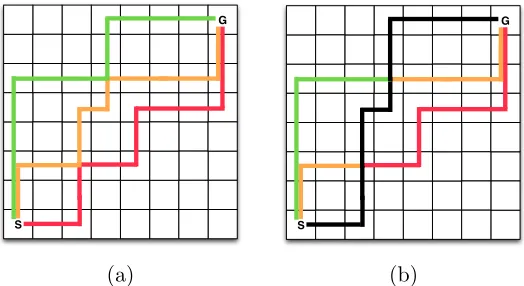
globally Pareto optimal. This process is highlighted in Figure 5 (a) where the state space is
optimal. To conclude, when in a state where multiple actions are considered non-dominated and therefore are incomparable, one can not randomly select between these actions when exploiting a chosen balance between criteria but actions need to be selected consistently.
S
G
S
G
(a) (b)
Figure 5: (a) In this environment, there is a green, yellow and red Pareto optimal action sequence that is globally optimal. (b) Selecting actions that are locally non-dominated within the current state does not guarantee that the entire policy is globally Pareto optimal. Hence, the information about the global Pareto front has been lost in the local Pareto front.
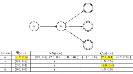
In order to solve the problem of locally optimal actions that are globally dominated, we define a globally greedy policy as a policyπ that consistentlyfollows ortracks a given expected return vectorVπ(s) from a statesso that its return equalsVπ(s) in expectation. Therefore, we need to retrieveπ, i.e., which actions to select from a start state to a terminal state. However, due to the stochastic behavior of the environment, it is not trivial to select the necessary actions so as to track the desired return vectors. Let us consider the small bi-objective MDP with deterministic transitions in Figure 6. When the agent reaches a terminal state, denoted by a double circle, the episode is finished. Assume that the discount factor γ is set to 1 for simplicity reasons. Once the Qset’s have converged separately, we can identify three Pareto optimal policies in the start states0. These policies
S0 a S1 b
c
d
Action R(s, a) N Dt(s, a) Qsetˆ (s, a)
a (0.2, 0.0) (0.9, 0.5), (2.0, 0.4), (0.0, 0.6)
(1.1, 0.5), (2.2, 0.4) , (0.2, 0.6)
b (0.9, 0.5) () (0.9, 0.5)
c (2.0, 0.4) () (2.0, 0.4)
d (0.0, 0.6) () (0.0, 0.6)
Figure 6: A small multi-objective MDP and its corresponding Qset’s. As we store the expected immediate and future non-dominated vectors separately, we can consis-tently follow expected return vectors from start to end state.
the environment and has to follow a particular policy so as to obtain the expected value of the policy from that state, i.e., Vπ(s), at the end of the episode. For each action of the action set A, we retrieve both the averaged immediate reward R(s, a) and N Dt(s, a), which we discount. If the sum of these two components equals the target vector to follow, we select the corresponding action and proceed to the next state. The return target to follow in the next states0 is then assigned toQ and the process continues until a terminal state is reached. When the vectors have not entirely converged yet or the transition scheme is stochastic, the equality operator at line 7 should be relaxed. In this case, the action is to be selected that minimizes the difference between the left and the right term. In our experiments, we select the action that minimizes the Manhattan distance between these terms.
4. Results and Discussion
Algorithm 7 Track policyπ given the expected reward vector Vπ(s) from states
1: target←Vπ(s)
2: repeat
3: for each ainAdo
4: Retrieve R(s, a)
5: Retrieve N Dt(s, a)
6: foreach Q inN Dt(s, a)do
7: if γQ+R(s, a) =targetthen
8: s←s0 :T(s0|s, a) = 1
9: target←Q
10: end if
11: end for
12: end for
13: untils is not terminal
framework in combination with the linear and Chebyshev scalarization function and the HB-MORL algorithm.
4.1 Performance Assessment of Multi-Policy Algorithms
In single-objective reinforcement learning, an algorithm is usually evaluated by its average reward accumulated over time. The curve of the graph then indicates both the speed of learning and the final performance of the converged policy. In multi-objective reinforcement learning, the performance assessment is more complex because of two main reasons: (1) the reward signal is vectorial and not scalar and (2) there exists no total ordering of the policies but there is a set ofincomparable optimal policies.
For scalarized MORL algorithms that converge to a single policy, Vamplew et al. (2010) propose to employ the hypervolume indicator on theapproximation set of policies, i.e., the policies that are obtained after applying a greedy policy for a range of experiments with varying parameters in the scalarization functions. The hypervolume of the approximation set can then be compared to the hypervolume of the true Pareto front, i.e., the set of Pareto optimal policies of the environment. Each experiment then represents an individual run of a scalarized MORL algorithm with a specific weight vectorw. In the case of tracking globally greedy policies, we can adopt the mechanism by Vamplew et al. (2010) and calculate the hypervolume of the cumulative reward vectors obtained by the tracking algorithm of Section 3.3 for each of the non-dominated vectors in theN D(∪aQsetˆ (s0, a)), wheres0 is the
start state. The hypervolume of each of these vectors should then approach the hypervolume of the Pareto front. It is important to note that in this way, we will evaluate and track as many policies as there exist non-dominated ˆQ-vectors in the start state for all actions.
4.2 Benchmarking Pareto Q-learning
with a linear, convex and non-convex Pareto front. All the experiments are averaged over 50 runs and their 95% confidence interval is depicted at regular intervals.
4.2.1 The Pyramid MDP
The Pyramid MDP is a new and simple multi-objective benchmark, which we introduce in this paper. A visual representation of the world is depicted in Figure 7 (a). The agent starts in the down-left position, denoted by a black dot at (0,0), and it can choose any of the four cardinal directions (up, down, left and right). The transition function is stochastic so that with a probability of 0.95 the selected action is performed and with a probability of 0.05 a random transition is executed to a neighboring state. The red dots represent terminal states. The reward scheme is bi-objective and returns a reward drawn from a Normal distribution withµ=−1 andσ = 0.01 for both objectives, unless a terminal state is reached. In that case, the x and y position of the terminal state is returned for the first and second objective, respectively. The Pareto front is therefore linear as depicted in Figure 7 (b).
0 10 20 30 40 50 60 70 80 90 100
0 10 20 30 40 50 60 70 80 90 100
X−axis
Y−axis
The Pyramid MDP
Non−terminal states Terminal states Start state
−20 0 20 40 60 80 100
−20 0 20 40 60 80 100
Objective 1
Objective 2
Pareto front of the Pyramid MDP
(a) (b)
Figure 7: The Pyramid MDP: the agent starts in the down-left position and can select actions until a terminal state is reached, denoted by a red dot. In (b), we represent the corresponding linear Pareto front.
As we are learning multiple policies simultaneously, which potentially may involve dif-ferent parts of the state space, we found it beneficial to employ a train and test setting, where in the train mode, we learn with an-greedy action selection strategy with decreas-ing epsilon.2 In the test mode of the algorithm, we perform multiple greedy policies using
Algorithm 7 for every element inN D(∪aQˆset(s0, a)) of the start states0 and we average the
accumulated returns along the paths. Each iteration, these average returns are collected and the hypervolume is calculated.
In Figure 8, we present the results of learning and sampling Pareto optimal policies in the Pyramid MDP environment for the train and test phases, respectively. In Figure 8 (a), we depict the hypervolume over time of the estimates in the start state s0.3 Hence,
2. At episodeeps, we assignedto be 0.997eps to allow for significant amounts of exploration in early runs
while maximizing exploitation in later runs of the experiment.
3. In the Pyramid MDP, the reference point for the hypervolume calculation in both HV-PQL and the
0 100 200 300 400 500 0
1000 2000 3000 4000 5000 6000 7000
Iteration
Hypervolume
Hypervolume of vectors in start state
PO−PQL C−PQL HV−PQL Pareto front
0 100 200 300 400 500
0 1000 2000 3000 4000 5000 6000 7000
Iteration
Hypervolume
Hypervolume of tracked policies of start state
PO−PQL C−PQL HV−PQL Pareto front
(a) (b)
0 20 40 60 80 100
0 0.1 0.2 0.3 0.4 0.5 0.6 0.7
Number of times the policy is tracked
Manhattan distance
Manhattan distance from sampled average to estimate
Manhattan distance
(c)
Figure 8: In (a), we depict the hypervolume of the estimates in the start state of the stochas-tic Pyramid MDP and we note that the entire Pareto front is learned very quickly during the learning phase. In (b), we track these estimates through the state space and denote that the hypervolume of their average returns approaches the Pareto front as well. In (c), we denote the performance of the tracking algorithm for a specific estimate. We see that the Manhattan distance of the running average of the return vector approaches the tracked estimate over time.
for each iteration, we calculate HV(∪aQˆset(s0, a)). We see that each of the set evaluation
multi-objective nature of the problem entails. Therefore, it treats every Pareto optimal solution equally and the estimates are updated much more consistently.
In Figure 8 (b), we depict the results of the tracking algorithm of Section 3.3 that globally follows every element of the start state in Figure 8 (a). We see that the hypervolume of the average returns of each the estimated ˆQ-vectors inN D(∪aQˆset(s, a)) is very similar to the learned estimates themselves. We see that tracking the estimates obtained by PO-PQL allows to sample the entire Pareto front over time.
In Figure 8 (c), we see the tracking algorithm at work to retrieve the policy of a specific vectorial estimate from the start state. In the figure, we denote the Manhattan distance of the running average return to the estimate after learning. We see that averaging the return of the policy obtained by the tracking algorithm over time approaches the estimate predicted at the start state, i.e., the distance becomes zero in the limit.
4.2.2 The Pressurized Bountiful Sea Treasure Environment
In order to evaluate the ParetoQ-learning algorithm on an environment with a larger num-ber of objectives, we propose the Pressurized Bountiful Sea Treasure (PBST) environment, which is inspired by the Deep Sea Treasure (DST) environment (Vamplew et al., 2010). Sim-ilar to the DST environment, the Pressurized Bountiful Sea Treasure environment concerns a deterministic episodic task where an agent controls a submarine, searching for undersea treasures. The world consists of a 10×11 grid where 10 treasures are located, with larger values as the distance from the starting location increases. A visualization of the envi-ronment is depicted in Figure 9 (a). At each time step, the agent can move into one of the cardinal directions. The goal of the agent is to minimize the time needed to reach the treasure, while maximizing the treasure value and to minimize the water pressure.4 The
pressure objective is a novel objective that was not included in the DST environment. It is defined as the agent’sy-coordinate. In contrast to the DST, the values of the treasures are altered to create a convex Pareto front. In the PBST environment, a Pareto optimal policy is a path to a treasure that minimizes the Manhattan distance while staying at the surface as long as possible before making the descent to retrieve a treasure. As a result, there are 10 Pareto optimal policies as shown in Figure 9 (b).
The results on the train and test phases are depicted in Figure 10 (a) and (b), respec-tively.5 In Figure 10 (b), we depict the hypervolume of the tracked policies of the start
state by applying the greedy policies. As the environment has both deterministic reward and transition schemes, the performance of the different set evaluation mechanisms is al-most identical. The tracking algorithm performs very well and the graph is alal-most identical to Figure 10 (a) as in the previous environment.
4. Traditionally, single-objective reinforcement learning solves a maximization problem. If the problem at hand concerns a minimization of one of the objectives, negative rewards are used for that objective to transform it also into a maximization problem.
5. In the PBST environment, the reference point for the hypervolume calculation in bothHV-PQLand the
−20 −15 −10 −5 0 0 50 100 150 200 −80 −60 −40 −20 0 Treasure objective Time objective Pressure objective (a) (b)
Figure 9: The Pressurized Bountiful Sea Treasure environment (a) and its Pareto front (b).
100 101 102 103
0 0.5 1 1.5 2 2.5 3 3.5
4x 10
5
Iteration
Hypervolume
Hypervolume of vectors in start state
PO−PQL C−PQL HV−PQL Pareto front
100 101 102 103
0 0.5 1 1.5 2 2.5 3 3.5
4x 10
5
Iteration
Hypervolume
Hypervolume of tracked policies of start state
PO−PQL C−PQL HV−PQL Pareto front
(a) (b)
Figure 10: The results on the PBST environment. In (a), we depict the hypervolume over time of the learned estimates in the start state. In (b), we see that the hyper-volume of the tracked policies is very similar to the hyperhyper-volume of the learned policies, which means that the learned policies are also retrievable.
4.3 Comparison to Single-Policy MORL Algorithms
In the previous section, we analyzed the performance of Pareto Q-learning in combina-tion with the three set evaluacombina-tion mechanisms . In this seccombina-tion, we conduct an empirical comparison of the algorithms to several single-policy MORL algorithms.
4.3.1 The Deep Sea Treasure Environment
−200 −18 −16 −14 −12 −10 −8 −6 −4 −2 0 20
40 60 80 100 120 140
Pareto front of the Deep Sea Treasure world
Time objective
Treasure objective
(a) (b)
Figure 11: Deep Sea Treasure environment (a) and its Pareto front (b).
The DST environment and its non-convex Pareto front are depicted in Figure 11 (a) and (b), respectively.
In Figure 12, we denote the hypervolume during the test phase of the algorithm with Pareto, cardinality and hypervolume set evaluations, i.e., PO-PQL, C-PQL and HV-PQL, respectively.6 Furthermore, we also evaluate two single-policy algorithms that employ the
linear and Chebyshev scalarization functions and HB-MORL, the indicator-based MORL algorithm of Section 2.2.1. These single-policy algorithms are evaluated using the config-uration specified in Section 4.1. Below, we highlight the performance of each algorithm individually.
The linear scalarized MORL algorithm is run with 10 uniformly distributed weight vectors, i.e., the continuous range of [0,1] is uniformly discretized with steps of 101−1 while satisfying Pm
o=1wo = 1. Each of these weights is then used in an individual execution of the scalarization algorithm and its results are collected in order to obtain a set of sampled policies in the test phase. We note that, although we have a uniform spread of weights, the algorithm only manages to retrieve a hypervolume of 768. When we take a closer look at the results obtained, we see that the algorithm learns fast but from iteration 200, only the optimal policies with return (−1,1) and (−19,124) for the time and treasure objectives, respectively, are sampled. This is shown by the 95% confidence intervals that become zero after iteration 200. This is to be expected as the Pareto front is non-convex and, hence, a linear combination of the objectives then can only differentiate between theextreme policies of the Pareto front. Therefore, the linear scalarized MORL algorithm converges to either of the optimal policies with return (−1,1) or (−19,124).
The Chebyshev scalarized MORL algorithm is equipped with the same set of weight vectors as the linear scalarization function. While the Chebyshev scalarization function has proven its effectiveness in multi-objective optimization, it is not guaranteed to converge to a Pareto optimal policy in a value-iteration approach (Perny and Weng, 2010). Nevertheless, we see that the algorithm performs acceptably in practice as it learns almost at the same speed as the linear scalarized MORL algorithm and attains a bigger hypervolume of 957. Other experiments will have to investigate whether this performance in practice is consistent over multiple environments, despite the lack of theoretical guarantees. A first initiative has been given in Van Moffaert et al. (2013b).
Although the indicator-based HB-MORL algorithm does not rely on any weighting pa-rameters, we also run the experiment 10 times in parallel to obtain a set of policies which we can compare at every time step. As there are no parameters to steer the search process, each individual experiment is not guaranteed to converge to a particular solution of the Pareto front. That is why the graph is increasing in the beginning of the learning process but it is slightly decreasing near the end as there is no mechanism, like for instance weights in the standard scalarization algorithms, to specify which experiment should focus on which part of the objective space. In the end, we see that the performance of HB-MORL drops slightly under the curve of the linear scalarized MORL algorithm.
So far, the single-policy algorithms did not manage to sample the entire Pareto front. This was a result of either the shape of the Pareto front, i.e., being non-convex, or the assignment of the weight vectors. Pareto Q-learning is not biased by any of these aspects, but treats every Pareto optimal solution equally in the bootstrapping process. As the environment consist of 10 Pareto optimal policies, the set of non-dominated vectors of the start state, i.e.,N D(∪aQˆset(s0, a)), exactly contains 10 elements. Therefore, we evaluate as
many policies as the scalarization algorithms in this comparison. In early learning phases, we see that for each of the set evaluation mechanisms, Pareto Q-learning learns slower than the scalarized MORL algorithms. This is because the weights of the scalarization algorithms guide each individual experiment to explore specific parts of the objective space, while the guidance mechanisms of the Pareto Q-learning algorithm, i.e., the set evaluation mechanisms, are less explicit. In the end, regardless of the set evaluation mechanisms used, Pareto Q-learning surpasses the performance of the single-policy algorithms. In this experiment, the Pareto set evaluation mechanism starts out the worst, but, in the end, it performs a bit better than the other set evaluation mechanisms and samples every element of the Pareto front.
5. Conclusions
In this paper, we have presented and discussed multi-objective optimization and reinforce-ment learning approaches for learning policies in multi-objective environreinforce-ments. We have highlighted that single-policy MORL algorithms rely on scalarization functions and weight vectors to translate the original multi-objective problem into a single-objective problem. Although these algorithms are very common in practice, they suffer from two main short-comings: their performance depends heavily on (1) the shape of the Pareto front and on (2) an appropriate choice of the weight vectors, which are hard to specify a priori.
The main contribution of this paper is the novel ParetoQ-learner algorithm that learns deterministic non-stationary non-dominated multi-objective policies for episodic environ-ments with a deterministic as well as stochastic transition function. To the best of our knowledge, PQL is the first multi-policy TD algorithm that allows to learn the entire Pareto front, and not just a subset. The core principle of our work consists of keeping track of the immediate reward vectors and the future discounted Pareto dominating vectors separately. This mechanism provides a neat and clean solution to update sets of vectors over time.
0 500 1000 1500 2000 2500 3000 0
200 400 600 800 1000 1200
Hypervolume of sampled policies in DST environment
Iteration
Hypervolume Pareto frontC−PQL
HV−PQL PO−PQL
Linear scalarized MORL Chebyshev scalarized MORL HB−MORL
Figure 12: The results on the Deep Sea Treasure environment. We compare three single-policy MORL algorithms that use a linear and Chebyshev scalarization function and HB-MORL to ParetoQ-learning with the three set evaluation mechanisms. We note that, regardless of the set evaluation mechanisms, PQL obtained better performance than the single-policy MORL algorithms and in the end PO-PQL sampled the entire Pareto front. For a more in-depth analysis of the results, we refer to Section 4.3.1.
The current set evaluation mechanisms rely on basic multi-objective indicators to translate the quality of a set of vectors into a scalar value. Based on these indications, local action selection is possible during the learning phase. Currently, we have combined PQL with a cardinality, hypervolume and Pareto indicator. We have seen that the Pareto indicator performed the best on average as it treats every Pareto optimal solution equally. The cardi-nality and hypervolume set evaluation measures rate the actions also on additional criteria than the Pareto relation to provide a total order. We have seen that in more complex environments, these set evaluation mechanisms bias the action selection too much in order to learn the entire Pareto front. Nevertheless, it could be that the user is not interested in sampling the entire Pareto front but is looking for particular policies that satisfy certain criteria. For instance, other quality indicators such as the spread indicator (Van Veld-huizen and Lamont, 1998) could be used to sample policies that are both Pareto optimal and well-spread in the objective space. This can straightforwardly be incorporated in our framework.
Pareto Q-learning’s performance to several single-policy MORL algorithms. We have seen that selecting actions that are locally dominating does not guarantee that the overall com-bination of selected actions in each state, i.e., the policy, is globally Pareto optimal. As a solution, we proposed a mechanism that tracks a given return vector, i.e., we can follow a selected expected return consistently from the start state to a terminal state in order to collect the predicted rewards.
In ParetoQ-learning, theQset’s grow according to the size of the Pareto front. Therefore, PQL is primarily designed for episodic environments with a finite number of Pareto optimal policies. To make the algorithm practically applicable for infinite horizon problems with a large value for the discount factor, we have to consider that all states can be revisited during the execution of an optimal policy. Upon revisiting a state, a different action that is optimal w.r.t. other criteria can be chosen. As explained by Mannor and Shimkin (2002), this offers a possibility to steer the average reward vector towards a target set using
approaching policies. Alternatively, we could reduce the number of learned policies by using
a consistency operator to select the same action during each revisit of some state, similar to the work of Wiering and de Jong (2007) for multi-criteria DP.
Currently, PQL is limited to a tabular representation where each state-action pair stores aQset. In order to make PQL applicable to real-life problems or ergodic environments, these sets should also be represented through function approximation. A possible idea is to fit the elements in each set through a geometric approach, such as for instance ordinal least-squares. If the environment would consist of two or three objectives, we would be fitting the vectors on a curve or a plane, respectively. In that case, we would be learning the shape of the Pareto front through local interactions that each update parts of this geometric shape. To summarize, we note that PQL (1) can learn the entire Pareto front under the as-sumption that each state-action pair is sufficiently sampled, (2) while not being biased by the shape of the Pareto front or a specific weight vector. Furthermore, we have seen that (3) the set evaluation mechanisms provide indicative measures to explore the objective space based on local action selections and (4) the learned policies can be tracked throughout the state and action space.
Acknowledgements
We would like to thank Tim Brys for his collaboration on the PBST environment and Diederik M. Roijers for his valuable insights and comments. This work has been carried out within the framework of the Perpetual project (grant nr. 110041) of the Institute for the Promotion of Innovation through Science and Technology in Flanders (IWT-Vlaanderen). Together with the Multi-Criteria Reinforcement Learning project (grant G.0878.14N) of the Fonds Wetenschappelijk Onderzoek - Vlaanderen (FWO).
References
L. Barrett and S. Narayanan. Learning all optimal policies with multiple criteria. In
Proceedings of the 25th International Conference on Machine Learning, ICML ’08, pages
N. Beume, B. Naujoks, and M. Emmerich. SMS-EMOA: multiobjective selection based on dominated hypervolume. European Journal of Operational Research, 181(3):1653–1669, September 2007.
C. A. C. Coello, G. B. Lamont, and D. A. V. Veldhuizen. Evolutionary Algorithms for
Solving Multi-Objective Problems (Genetic and Evolutionary Computation).
Springer-Verlag New York, Inc., Secaucus, NJ, USA, 2006. ISBN 0387332545.
I. Das and J. E. Dennis. A closer look at drawbacks of minimizing weighted sums of objectives for Pareto set generation in multicriteria optimization problems. Structural
and Multidisciplinary Optimization, 14:63–69, 1997. ISSN 1615-147X.
K. D. Deb, A. Pratap, S. Agarwal, and T. Meyarivan. A fast and elitist multiobjective genetic algorithm : NSGA-II. IEEE Transactions on Evolutionary Computation, 6(2): 182–197, April 2002. ISSN 1089778X. doi: 10.1109/4235.996017.
N. Dunford, J. T. Schwartz, W. G. Bade, and R. G. Bartle. Linear Operators: General
theory. Part. I. Linear Operators. Interscience Publishers, 1988. ISBN 9780470226056.
Z. Gabor, Z. Kalmar, and C. Szepesvari. Multi-criteria reinforcement learning. In
Proceed-ings of the 15th International Conference on Machine Learning, ICML ’98, Madison, WI,
1998.
J.-M. Gorce, R. Zhang, K. Jaffr`es-Runser, and C. Goursaud. Energy, latency and capacity trade-offs in wireless multi-hop networks. In Proceedings of the IEEE 21st International
Symposium on Personal, Indoor and Mobile Radio Communications, PIMRC 2010, pages
2757–2762. IEEE, 2010.
F. Hernandez-del Olmo, F. H. Llanes, and E. Gaudioso. An emergent approach for the control of wastewater treatment plants by means of reinforcement learning techniques.
Expert Systems with Applications, 39(3):2355–2360, 2012.
C. Igel, N. Hansen, and S. Roth. Covariance matrix adaptation for multi-objective opti-mization. Evolutionary Computation, 15(1):1–28, 2007.
D. J. Lizotte, M. Bowling, and S. A. Murphy. Efficient reinforcement learning with multiple reward functions for randomized controlled trial analysis. In Proceedings of the
Twenty-Seventh International Conference on Machine Learning, ICML ’10, pages 695–702, 2010.
D. J. Lizotte, M. Bowling, and S. A. Murphy. Linear fitted-q iteration with multiple reward functions. Journal of Machine Learning Research, 13:3253–3295, 2012.
S Mannor and N. Shimkin. The steering approach for multi-criteria reinforcement learn-ing. In T.G. Dietterich, S. Becker, and Z. Ghahramani, editors, Advances in Neural
Information Processing Systems 14, pages 1563–1570. MIT Press, 2002.
S. Mannor and N. Shimkin. A geometric approach to multi-criterion reinforcement learning.
K. Miettinen and M. M. M¨akel¨a. On scalarizing functions in multiobjective optimization.
OR Spectrum, 24:193–213, 2002. ISSN 0171-6468.
P. Perny and P. Weng. On finding compromise solutions in multiobjective Markov decision processes. InProceedings of the 19th European Conference on Artificial Intelligence, ECAI ’10, pages 969–970, Amsterdam, The Netherlands, 2010. IOS Press. ISBN 978-1-60750-605-8.
D. M. Roijers, P. Vamplew, S. Whiteson, and R. Dazeley. A survey of multi-objective sequential decision-making. Journal of Artificial Intelligence Research, 48:67–113, 2013.
R. S. Sutton and A. G. Barto. Reinforcement Learning: An Introduction. Adaptive Com-putation and Machine Learning. Mit Press, 1998. ISBN 9780262193986.
G. Tesauro, R. Das, H. Chan, J. O. Kephart, D. W. Levine, F. Rawson, and C. Lefurgy. Managing power consumption and performance of computing systems using reinforcement learning. In J.C. Platt, D. Koller, Y. Singer, and S.T. Roweis, editors,Advances in Neural
Information Processing Systems 20, pages 1497–1504. Curran Associates, Inc., 2008.
J. N. Tsitsiklis. Asynchronous stochastic approximation and q-learning.Journal of Machine
Learning, 16(3):185–202, 1994.
P. Vamplew, J. Yearwood, R. Dazeley, and A. Berry. On the limitations of scalarisation for multi-objective reinforcement learning of Pareto fronts. In Proceedings of the 21st
Aus-tralasian Joint Conference on Artificial Intelligence: Advances in Artificial Intelligence,
AI ’08, pages 372–378, Berlin, Heidelberg, 2008. Springer-Verlag. ISBN 978-3-540-89377-6.
P. Vamplew, R. Dazeley, E. Barker, and A. Kelarev. Constructing stochastic mixture policies for episodic multiobjective reinforcement learning tasks. In A. E. Nicholson and X. Li, editors,Australasian Conference on Artificial Intelligence, volume 5866 of Lecture
Notes in Computer Science, pages 340–349. Springer, 2009. ISBN 978-3-642-10438-1.
P. Vamplew, R. Dazeley, A. Berry, R. Issabekov, and E. Dekker. Empirical evaluation methods for multiobjective reinforcement learning algorithms. Machine Learning, 84 (1-2):51–80, 2010.
K. Van Moffaert, M. M. Drugan, and A. Now´e. Hypervolume-based multi-objective rein-forcement learning. In R. Purshouse, P. Fleming, C. Fonseca, S. Greco, and J. Shaw, editors, Evolutionary Multi-Criterion Optimization, volume 7811 of Lecture Notes in
Computer Science, pages 352–366. Springer Berlin Heidelberg, 2013a. ISBN
978-3-642-37139-4.
K. Van Moffaert, M. M Drugan, and A. Now´e. Scalarized multi-objective reinforcement learning: Novel design techniques. In 2013 IEEE International Symposium on Adaptive
Dynamic Programming And Reinforcement Learning (ADPRL), pages 191–199. IEEE,
D. A. Van Veldhuizen and G. B. Lamont. Multiobjective evolutionary algorithm research: a history and analysis. Technical Report TR-98-03, Department of Electrical and Computer Engineering, Graduate School of Engineering, Air Force Institute of Technology, Wright-Patterson AFB, Ohio, 1998.
W. Wang and M. Sebag. Hypervolume indicator and dominance reward based multi-objective Monte-Carlo tree search. Machine Learning, 92(2-3):403–429, 2013. ISSN 0885-6125. doi: 10.1007/s10994-013-5369-0.
C. Watkins.Learning from Delayed Rewards. PhD thesis, University of Cambridge, England, 1989.
D. J. White. Multi-objective infinite-horizon discounted Markov decision processes. Journal
of Mathematical Analysis and Applications, 89(2), 1982.
M. A. Wiering and E. D. de Jong. Computing optimal stationary policies for multi-objective Markov decision processes. In 2007 IEEE International Symposium on Approximate
Dynamic Programming and Reinforcement Learning, pages 158–165. IEEE, April 2007.
ISBN 1-4244-0706-0.
E. Zitzler, M. Laumanns, and L. Thiele. SPEA2: Improving the strength Pareto evolu-tionary algorithm for multiobjective optimization. In K.C. Giannakoglou et al., editors,
Evolutionary Methods for Design, Optimisation and Control with Application to Industrial
Problems (EUROGEN 2001), pages 95–100. International Center for Numerical Methods
in Engineering (CIMNE), 2002.
E. Zitzler, L. Thiele, M. Laumanns, C. M. Fonseca, and V. Grunert da Fonseca. Performance assessment of multiobjective optimizers: An analysis and review. IEEE Transactions on