Penalized Maximum Likelihood Estimation of
Multi-layered Gaussian Graphical Models
Jiahe Lin ∗ [email protected]
Department of Statistics University of Michigan Ann Arbor, MI 48109, USA
Sumanta Basu ∗ [email protected]
Department of Statistics
University of California, Berkeley Berkeley, CA 94720, USA
Moulinath Banerjee [email protected]
Department of Statistics University of Michigan Ann Arbor, MI 48109, USA
George Michailidis † [email protected]
Department of Statistics and Computer & Information Science & Engineering University of Florida
Gainesville, FL 32611, USA
Editor:Jie Peng
Abstract
Analyzing multi-layered graphical models provides insight into understanding the con-ditional relationships among nodes within layers after adjusting for and quantifying the effects of nodes from other layers. We obtain the penalized maximum likelihood estimator for Gaussian multi-layered graphical models, based on a computational approach involving screening of variables, iterative estimation of the directed edges between layers and undi-rected edges within layers and a final refitting and stability selection step that provides improved performance in finite sample settings. We establish the consistency of the es-timator in a high-dimensional setting. To obtain this result, we develop a strategy that leverages the biconvexity of the likelihood function to ensure convergence of the developed iterative algorithm to a stationary point, as well as careful uniform error control of the esti-mates over iterations. The performance of the maximum likelihood estimator is illustrated on synthetic data.
Keywords: graphical models, penalized likelihood, block coordinate descent, conver-gence, consistency
∗. Equal Contribution
1. Introduction.
The estimation of directed and undirected graphs from high-dimensional data has received a lot of attention in the machine learning and statistics literature (e.g., see B¨uhlmann and Van De Geer,2011, and references therein), due to their importance in diverse applications including understanding of biological processes and disease mechanisms, financial systems stability and social interactions, just to name a few (Sachs et al.,2005;Wang et al., 2007; Sobel,2000). In the case of undirected graphs, the edges capture conditional dependence relationships between the nodes, while for directed graphs they are used to model causal relationships (B¨uhlmann and Van De Geer,2011).
However, in a number of applications the nodes can be naturally partitioned into sets that exhibit interactions both between them and amongst them. As an example, consider an experiment where one has collected data for both genes and metabolites for the same set of patient specimens. In this case, we have three types of interactions between genes and metabolites: regulatory interactions between the two of them and co-regulation within the gene and within the metabolic compartments. The latter two types of relationships can be expressed through undirected graphs within the sets of genes and metabolites, respectively, while the regulation of metabolites by genes corresponds to directed edges. Note that in principle there are feedback mechanisms from the metabolic compartment to the gene one, but these are difficult to detect and adequately estimate in the absence of carefully collected time course data. Another example comes from the area of financial economics, where one collects data on returns of financial assets (e.g. stocks, bonds) and also on key macroeconomic indicators (e.g. interest rate, prices indices, various measures of money supply and various unemployment indices). Once again, over short time periods there is influence from the economic variables to the returns (directed edges), while there are co-dependence relationships between the asset returns and the macroeconomic variables, respectively, that can be modeled as undirected edges.
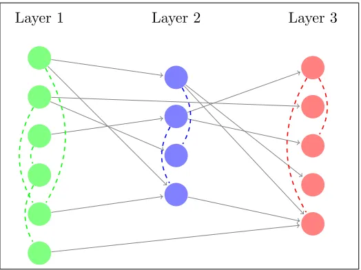
Technically, such layered network structures correspond to multi-partite graphs that possess undirected edges and exhibit a directed acyclic graph structure between the layers, as depicted in Figure1, where we use directed solid edges to denote the dependencies across layers and dashed undirected edges to denote within-layer conditional dependencies.
Selected properties of such so-calledchain graphshave been studied in the work ofDrton and Perlman(2008), with an emphasis on two alternative Markov properties including the LWF Markov property (Lauritzen and Wermuth, 1989; Frydenberg, 1990) and the AMP Markov property (Andersson et al.,2001).
Layer 2
Layer 1 Layer 3
Figure 1: Diagram for a three-layered network
However, this method does not scale well according to the simulation results presented and no theoretical properties of the estimates were provided.
In follow-up work, Yin and Li(2011) used a cyclic block coordinate descent algorithm and claimed convergence to a stationary point leveraging a result in Tseng (2001) (see Proposition 2 in the Supplemental material). Unfortunately, a key assumption in Tseng (2001) -namely, that a corresponding coordinate wise optimization problem that is given by a high-dimensional lasso regression has unique minimum- fails and hence the convergence result does not go through.
In related work, Lee and Liu(2012) proposed the Plug-in Joint Weighted Lasso (PWL) and the Plug-in Joint Graphical Weighted Lasso (PWGL) estimator for estimating the same 2-layered structure, where they use a weighted version of the algorithm inRothman et al. (2010) and also provide theoretical results for the low dimensional setting, where the number of samples exceeds the number of potential directed and undirected edges to be estimated. Finally, Cai et al. (2012) proposed a method for estimating the same 2-layered structure and provided corresponding theoretical results in the high dimensional setting. The Dantzig-type estimator (Candes and Tao,2007) was used for the regression coefficients and the corresponding residuals were used as surrogates, for obtaining the precision matrix through the CLIME estimator (Cai et al.,2011). In another line of work (Sohn and Kim, 2012; Yuan and Zhang, 2014; McCarter and Kim, 2014), structured sparsity of directed edges was considered and the edges were estimated with a different parametrization of the objective function. We further elaborate on the connections of our work with these three papers in Section 5.
esti-mate the homogeneous and heterogeneous neighborhood for each node, by obtaining the`1 regularized M-estimator of the node-conditional distribution parameters, using traditional approaches (e.g. Meinshausen and B¨uhlmann, 2006) for neighborhood estimation. How-ever, rather than estimating directed edges directly, the directed edges are obtained from a nonlinear transformation of the estimated homogeneous and heterogeneous neighborhood, whose sparsity pattern gets compromised during the process.
In this work, we obtain the regularized maximum likelihood estimator under a spar-sity assumption on both directed and undirected parameters for multi-layered Gaussian graphical models and establish its consistency properties in a high-dimensional setting. As discussed in Section 3, the problem isnot jointly convex on the parameters, but convex on selected subsets of them. Further, it turns out that the problem isbiconvex if we consider a recursive multi-stage estimation approach that at each stage involves only regression param-eters (directed edges) from preceding layers and precision matrix paramparam-eters (undirected edges) for the last layer considered in that stage. Hence, we decompose the multi-layer network structure estimation into a sequence of 2-layer problems that allows us to estab-lish the desired results. Leveraging the biconvexity of the 2-layer problem, we estabestab-lish the convergence of the iterates to the maximum-likelihood estimator, which under certain regularity conditions is arbitrarily close to the true parameters. The theoretical guarantees provided require a uniform control of the precision of the regression and precision matrix parameters, which poses a number of theoretical challenges resolved in Section 3.
In summary, despite the lack of overall convexity, we are able to provide theoretical guarantees for the MLE in a high dimensional setting. We believe that the proposed strategy is generally applicable to other non-convex statistical estimation problems that can be decomposed to two biconvex problems. Further, to enhance the numerical performance of the MLE in finite (and small) sample settings, we introduce a screening step that selects active nodes for the iterative algorithm used and that leverages recent developments in the high-dimensional regression literature (e.g., Van de Geer et al., 2014; Javanmard and Montanari, 2014; Zhang and Zhang, 2014). We also post-process the final MLE estimate through a stability selection procedure. As mentioned above, the screening and stability selection steps are beneficial to the performance of the MLE in finite samples and hence recommended for similarly structured problems.
2. Problem Formulation.
Consider anM-layered Gaussian graphical model. Suppose there arepm nodes in Layerm,
denoted by
Xm= (X1m,· · · , Xpmm)0, form= 1,· · ·, M. The structure of the model is given as follows:
– Layer 1. X1 = (X11,· · · , Xp11)0∼ N(0,Σ1).
– Layer 2. For j = 1,· · · , p2: Xj2 = (Bj12)0X1 + 2j, with B12j ∈ Rp1, and 2 =
(2
1,· · · , 2p2)
0 ∼ N(0,Σ2). ..
.
– LayerM. Forj= 1,2,· · · , pM:
XjM =
M−1
X
m=1
{(BjmM)0Xm}+Mj , whereBjmM ∈Rpm form= 1,· · ·, M −1,
and M = (M1 ,· · · , MpM)0 ∼ N(0,ΣM).
The parameters of interest areall directed edgesthat encode the dependencies across layers, that is,
Bst :=B1st · · · Bpstt, for 1≤s < t≤M,
and all undirected edges that encode the conditional dependencies within layers after ad-justing for the effects from directed edges, that is:
Θm:= (Σm)−1, form= 1,· · ·, M.
It is assumed thatBst and Θm aresparse for all 1, . . . , M and 1≤s < t≤M.
Given centered data for all M layers, denoted by Xm= [X1m,· · · , Xpmm]∈Rn×pm for all m = 1,· · ·, M, we aim to obtain the MLE for all Bst,1 ≤ s < t ≤ M and all Θm, m =
1,· · · , M parameters. Henceforth, we useXm to denote random vectors, andXjm to denote thejth column in the data matrix Xnm×pm whenever there is no ambiguity.
Through Markov factorization (Lauritzen,1996), the full log-likelihood function can be decomposed as
`(Xm;Bst,Θm,1≤s < t≤M,1≤m≤M) =`(XM|XM−1,· · ·, X1;B1M,· · ·, BM−1,M,ΘM)
+`(XM−1|XM−2,· · ·, X1;B1M−1,· · ·, BM−2,M−1,ΘM−1) +· · ·+`(X2|X1;B12,Θ2) +`(X1; Θ1)
=`(X1; Θ1) +XM
m=2`(X
combined as a super “parent” layer. If we ignore the structure within the bottom layer (X1) for the moment, theM-layered network can be viewed as (M−1) two-layered networks, each comprising a response layer and a parent layer. Thus, the network structure in Figure1can be viewed as a 2 two-layered network: for the first network, Layer 3 is the response layer, while Layers 1 and 2 combined form the “parent” layer; for the second network, Layer 2 is the response layer, and Layer 1 is the “parent” layer. Therefore, the problem for estimating all M2
coefficient matrices and M precision matrices can be translated into estimating (M −1) two-layered network structures with directed edges from the parent layer to the response layer, and undirected edges within the response layer, and finally estimating the undirected edges within the bottom layer separately.
Since all estimation problems boil down to estimating the structure of a 2-layered net-work, we focus the technical discussion on introducing our proposed methodology for a 2-layered network setting,1. The theoretical results obtained extend in a straightforward manner to an M-layered Gaussian graphical model.
Remark 1. For theM-layer network structure, we impose certain identifiability-type condi-tion on the largest “parent” layer (encompassingM −1 layers), so that the directed edges of the entire network are estimable. The imposed condition translates into a minimum eigenvalue-type condition on the population precision matrix within layers, and conditions on the magnitude of dependencies across layers. Intuitively, consider a three-layered net-work: ifX1 andX2 are highly correlated, then the proposed (as well as any other) method will exhibit difficulties in distinguishing the effect of X1 on X3 from that of X2 on X3. The (group) identifiability-type condition is thus imposed to obviate such circumstances. An in-depth discussion on this issue is provided in Section3.4.
2.1 A Two-layered Network Setup.
Consider a two-layered Gaussian graphical model with p1 nodes in the first layer, denoted by X = (X1,· · · , Xp1)
0, and p
2 nodes in the second layers, denoted by Y = (Y1,· · · , Yp2)
0.
The model is defined as
– X = (X1,· · ·, Xp1)
0 ∼ N(0,Σ
X).
– Forj= 1,2,· · ·, p2: Yj =Bj0X+j,Bj ∈Rp1 and = (1,· · · , p2)
>∼ N(0,Σ
).
The parameters of interest are: ΘX := Σ−X1,Θ := Σ−1 and B = [B1,· · ·, Bp2]. As with
most estimation problems in the high dimensional setting, we assume these parameters to be sparse.
Now given data X = [X1,· · ·, Xp1]∈ R
n×p1 and Y = [Y1,· · ·, Y
p2]∈R
n×p2, both
cen-tered, we would like to use the penalized maximum likelihood approach to obtain estimates for ΘX, Θ andB. Throughout this paper, we use X,Y andE to denote the size-n
realiza-tions of the random vectorsX,Y and, respectively. Also, with a slight abuse of notation, we useXi, i= 1,2,· · ·, p1 andYj, j = 1,2,· · ·, p2 to denote the columns of the data matrix
X and Y, respectively, whenever there is no ambiguity.
The full log-likelihood can be written as
`(X, Y;B,Θ,ΘX) =`(Y|X; Θ, B) +`(X; ΘX) (1)
Note that the first term only involves Θ and B, and the second term only involves ΘX.
Hence, (1) can be maximized by maximizing `(Y|X) w.r.t. (Θ, B), and maximizing `(X)
w.r.t. ΘX, respectively. ΘbX can be obtained using traditional methods for estimating
undirected graphs, e.g., the Graphical Lasso (Friedman et al., 2008) or the Nodewise Re-gression prcoedure (Meinshausen and B¨uhlmann, 2006). Therefore, the rest of this paper will mainly focus on obtaining estimates for ΘandB. In the next subsection, we introduce
our estimation procedure for obtaining the MLE for Θ and B.
Remark 2. Our proposed method is targeted towards maximizing `(Y|X; Θ, B) (with
proper penalization) in (1) only, which gives the estimates for across-layers dependencies between the response layer and the parent layer, as well as estimates for the conditional dependencies within the response layer each time we solve a 2-layered network estimation problem. For an M-layered estimation problem, the maximization regarding `(X; ΘX)
oc-curs only when we are estimating the within-layer conditional dependencies for the bottom layer.
2.2 Estimation Algorithm.
The conditional likelihood for response Y givenX can be written as
L(Y|X) = (√1
2π) np2|Σ
⊗In|−1/2exp
−12(Y − Xβ)>(Σ⊗In)−1(Y − Xβ) ,
whereY =vec(Y1,· · ·, Yp2), X =Ip2⊗X andβ =vec(B1,· · ·, Bp2). After writing out the
Kronecker product, the log-likelihood can be written as
`(Y|X) = constant +n
2 log det Θ− 1 2
p2
X
j=1
p2
X
i=1
σij(Yi−XBi)>(Yj−XBj).
Here, σij denotes the ij-th entry of Θ. With `1 penalization which induces sparsity, we
formulate the following optimization problem using penalized log-likelihood, which was initially proposed in Rothman et al. (2010), and has also been examined in Lee and Liu (2012):
min
B∈Rp1×p2
Θ∈Sp++2×p2
1 n
p2
X
j=1
p2
X
i=1
σij(Yi−XBi)>(Yj−XBj)−log det Θ+λn p2
X
j=1
kBjk1+ρnkΘk1,off
,
(2) and the first term in (2) can be equivalently written as
tr
1
n
(Y1−XB1)> .. . (Yp2 −XBp2)
>
(Y1−XB1) · · · (Yp2 −XBp2)
Θ
whereS is defined as the sample covariance matrix ofE ≡Y −XB. This gives rise to the following optimization problem:
min
B∈Rp1×p2
Θ∈Sp++2×p2
tr(SΘ)−log det Θ+λn p2
X
j=1
kBjk1+ρnkΘk1,off
≡f(B,Θ), (3)
where kΘk1,off is the absulote sum of the off-diagonal entries in Θ, λn and ρn are both
positive tuning parameters.
Note that the objective function (3) is not jointly convex in (B,Θ), but only convex
in B for fixed Θ and in Θ for fixedB; hence, it is bi-convex, which in turn implies that
the proposed algorithm may fail to converge to the global optimum, especially in settings wherep1 > n, as pointed out by Lee and Liu (2012). As is the case with most non-convex problems, good initial parameters are beneficial for fast convergence of the algorithm, a fact supported by our numerical work on the present problem. Further, a good initialization is critical in establishing convergence of the algorithm for this problem (see Section3.1). To that end, we introduce a screening step for obtaining a good initial estimate for B. The theoretical justification for employing the screening step is provided in Section 3.3.
An outline of the computational procedure is presented in Algorithm1, while the details of each step involved are discussed next.
Screening. For each variable Yj, j = 1,· · ·, p2 in the response layer, regress Yj on X
via the de-biased Lasso procedure proposed by Javanmard and Montanari (2014). The output consists of the p-value(s) for each predictor in each regression, denoted by Pj, with
Pj ∈ [0,1]p1. To control the family-wise error rate of the estimates, we do a Bonferroni
correction at level α: define α? =α/p
1p2 and setBj,k = 0 if the p-value obtained for the
k’th predictor in the j’th regressionPj,k exceeds α?. Further, let
Bj ={Bj ∈Rp1 :Bj,k = 0 if k∈Sbjc} ⊆Rp1, (4)
whereSbj is the collection of indices for those predictors deemed “active” for responseYj:
b
Sj ={k:Pj,k < α?}, forj= 1,· · ·, p2.
Therefore, subsequent estimation of the elements ofB will be restricted toB1× · · · × Bp2.
Alternating Search. In this step, we utilize the bi-convexity of the problem and estimate Band Θby minimizing in an iterative fashion the objective function with respect to (w.r.t.)
one set of parameters, while holding the other set fixed within each iteration.
As with most iterative algorithms, we need an initializer; for Bb(0) it corresponds to a
Lasso/Ridge regression estimate with a small penalty, while for Θb we use the Graphical
Lasso procedure applied to the residuals obtained from the first stage regression. That is, for each j= 1,· · ·, p2,
b
Bj(0)= argmin
Bj∈Bj
Algorithm 1:Computational procedure for estimating B and Θ
Input : Data from the parent layer X and the response layer Y.
1 Screening:
2 forj= 1,· · · , p2 do
regress Yj on X using the de-biased Lasso procedure inJavanmard and Montanari
(2014) and obtain the corresponding vector of p-valuesPj;
end
obtain adjusted p-valuesPej by applying Bonferroni correction to vec(P1,· · ·, Pj);
determine the support setBj for each regression using (4).
3 Initialization:
4 Initialize columnj= 1,· · ·, p2 of Bb(0) by solving (5).
InitializeΘb
(0)
by solving (9) using the graphical lasso (Friedman et al.,2008).
5 while |f(Bb(k),Θb
(k)
)−f(Bb(k+1),Θb
(k+1)
)| ≥do
6 updateBb with (6);
7 updateΘb with (8);
8 end
9 Refitting B and Θ: forj= 1,· · · , p2 do
Obtain the refittedBej using (9);
end
re-estimate Θe using (10) withW coming from stability selection.
Output: Final Estimates Be and Θe.
whereλ0n is some small tuning parameter for initialization, and setEb
(0)
j :=Yj−XBb
(0)
j . An
initial estimate for Θb is then given by solving for the following optimization problem with
the graphical lasso (Friedman et al.,2008) procedure:
b
Θ(0) = argmin Θ∈Sp2×p2
++
n
log det Θ−tr(Sb(0)Θ) +ρnkΘk1,off o
,
whereSb(0) is the sample covariance matrix based on (Eb
(0)
1 ,· · · ,Eb
(0)
p2 ).
Next, we use an alternating block coordinate descent algorithm with `1 penalization to reach a stationary point of the objective function (3).
– UpdateB as
b
B(k+1) = argmin
B∈B1×···×Bp2
1 n
p2
X
i=1
p2
X
j=1
(bσij )(k)(Yi−XBi)>(Yj −XBj) +λn p2
X
j=1
kBjk1
,
which can be obtained by cyclic coordinate descent w.r.t each column Bj of B, that
is, update each columnBj by:
b
Bj(t+1)= argmin
Bj∈Bj
n
(bσjj)(k)
n kYj +r
(t+1)
j −XBjk22+λnkBjk1
o
, (7)
where
rj(t+1) = 1 (σbjj )(k)
j−1
X
i=1
(bσij)(k)(Yi−XBb
(t+1)
i ) +
p2
X
i=j+1
(σbij )(k)(Yi−XBb
(t)
i )
,
and iterate over all columns until convergence. Here, we use k to index the outer iteration while minimizing w.r.t. B or Θ, and usetto index the inner iteration while
cyclically minimizing w.r.t. each column of B.
– Update Θ as
b
Θ(k+1)= argmin Θ∈Sp2×p2
++
n
log det Θ−tr(Sb(k+1)Θ) +ρnkΘk1,off o
, (8)
where Sb(k+1) is the sample covariance matrix based on Eb
(k+1)
j = Yj −XBb
(k+1)
j , j =
1,· · · , p2.
Refitting and Stabilizing. As noted in the introduction, this step is beneficial in applica-tions, especially when one deals with large scale multi-layer networks and relatively smaller sample sizes. Denote the solution obtained by the above iterative procedure by B∞ and Θ∞ . For each j = 1,· · ·, p2, set Bej ={Bj :Bj,i = 0 if Bj,i∞ = 0, Bj ∈ Rp1} and the final
estimate for Bj is given by ordinary least squares:
e
Bj = argmin Bj∈Bej
kYj−XBjk2. (9)
For Θ, we obtain the final estimate by a combination of stability selection (Meinshausen and
B¨uhlmann, 2010) and graphical lasso (Friedman et al.,2008). That is, after obtaining the refitted residuals Eej :=Yj−XBej, j = 1,· · · , p2, based on the stability selection procedure
with the graphical lasso, we obtain the stability path, or probability matrixW for each edge, which records the proportion of each edge being selected based on bootstrapped samples of Eej’s. Then, using this probability matrix W as a weight matrix, we obtain the final
estimate ofΘe as follow:
e
Θ= argmin
Θ∈Sp++2×p2
n
log det Θ−tr(SΘe ) +ρenk(1−W)∗Θk1,off o
, (10)
where we use ∗ to denote the element-wise product of two matrices, and Se is the sample
covariance matrix based on the refitted residuals E. Again, (e 10) can be solved by the
2.3 Tuning Parameter Selection.
To select the tuning parameters (λn, ρn), we use the Bayesian Information Criterion(BIC),
which is the summation of a goodness-of-fit term (log-likelihood) and a penalty term. The explicit form of BIC (as a function of B and Θ) in our setting is given by
BIC(B,Θ) =−log det Θ+ tr(SΘ) +
logn n (
kΘk0−p2
2 +kBk0) where
S:= 1 n
(Y1−XB1)> .. . (Yp2−XBp2)
>
(Y1−XB1) · · · (Yp2 −XBp2)
,
and kΘk0 is the total number of nonzero entries in Θ. Here we penalize the non-zero
elements in the upper-triangular part of Θ and the non-zero ones in B. We choose the
combination (λ∗n, ρ∗n) over a grid of (λ, ρ) values, and (λ∗n, ρ∗n) should minimize the BIC evaluated at (B∞,Θ∞ ).
3. Theoretical Results.
In this section, we establish a number of theoretical results for the proposed iterative al-gorithm. We focus the presentation on the two-layer structure, since as explained in the previous section the multi-layer estimation problem decomposes to a series of two-layer ones. As mentioned in the introduction, one key challenge for establishing the theoretical results comes from the fact that the objective function (3) is not jointly convex in B and Θ. Consequently, if we simply used properties of block-coordinate descent algorithms, we
would not be able to provide the necessary theoretical guarantees for the estimates we ob-tain. On the other hand, the biconvex nature of the objective function allows us to establish convergence of the alternating algorithm to a stationary point, provided it is initialized from a point close enough to the true parameters. This can be accomplished using a Lasso-based initializer forB and Θ as previously discussed. The details of algorithmic convergence are
presented in Section 3.1.
Another technical challenge is that each update in the alternating search step relies on estimated quantities—namely the regression and precision matrix parameters—rather than the raw data, whose estimation precision needs to be controlled uniformly across all iterations. The details of establishing consistency of the estimates for both fixed and random realizations are given in Section 3.2.
Next, we outline the structure of this section. In Section3.1Theorem1, we show that for any fixed set of realization ofX andE,2 the iterative algorithm is guaranteed to converge to a stationary point if estimates for all iterations lie in a compact ball around the true value of the parameters. In Section 3.2, we show in Theorem 4 that for any random X and E, with high probability, the estimates for all iterations lie in a compact ball around the true value of the parameters. Then in Section 3.3, we show that asymptotically with
log(p1p2)/n→0, while keeping the family-wise type I error under some pre-specified level, the screening step correctly identifies the true support set for each of the regressions, based upon which the iterative algorithm is provided with an initializer that is close to the true value of the parameters. Finally in Section 3.4, we provide sufficient conditions for both directed and undirected edges to be identifiable (estimable) for multi-layered network.
To aid the readability of the main results, we only present statements of theorems and propositions, while all proofs are relegated to the Appendix (Section A andB).
Throughout this section, to distinguish the estimates from the true values, we use B∗ and Θ∗ to denote the true values.
3.1 Convergence of the Iterative Algorithm.
In this subsection, we prove that the proposed block relaxation algorithm converges to a stationary point for any fixed set of data, provided that the estimates for all iterations lie in a compact ball around the true value of the parameters. This requirement is shown to be satisfied with high probability in the next subsection 3.2.
Decompose the optimization problem in (3) as follows:
min
B∈Rp1×p2
Θ∈Sp++2×p2
f(B,Θ)≡f0(B,Θ) +f1(B) +f2(Θ),
where
f0(B,Θ) =
1 n
p2
X
j=1
p2
X
i=1
σij (Yi−XBi)0(Yj−XBj)−log det Θ= tr(SΘ)−log det Θ,
f1(B) =λnkBk1, f2(Θ) =ρnkΘk1,off.
andSp++2×p2 is the collection ofp2×p2 symmetric positive definite matrices. Further, denote the limit point (if there is any) of {Bb(k)} and {Θb
(k)
} by B∞ = limk→∞Bb(k) and Θ∞ =
limk→∞Θb
(k)
, respectively.
Definition 1(stationary point (Tseng,2001) pp.479). Definez to be a stationary point of f ifz∈dom(f) andf0(z;d)≥0,∀direction d= (d1,· · · , dN) wheredtis thetth coordinate
block.
Definition 2 (Regularity (Tseng,2001) pp.479). f is regular atz∈dom(f) iff0(z;d)≥0 for all d= (d1,· · · , dN) such that
f0(z; (0,· · ·, dt,· · · ,0))≥0, t= 1,2,· · ·, N.
Definition 3 (Coordinate-wise minimum). Define (B∞,Θ∞ ) to be a coordinate-wise min-imum if
f(B∞,Θ) ≥ f(B∞,Θ∞), ∀Θ∈Sp++2×p2, f(B,Θ∞ ) ≥ f(B∞,Θ∞ ), ∀B ∈Rp1×p2.
Remark 3. Tseng (2001) proved that if the level set {x :f(x) ≤f(x0)} is compact and f satisfies certain conditions (Tseng, 2001, see Theorem 4.1 (a), (b) and (c) for details), the limit point given by the general block-coordinate descent algorithm (withN ≥2 blocks) is a stationary point off. However, the conditions given in Theorem 4.1 (a), (b) and (c) are not satisfied for the objective function at hand. Hence, for the problem under consideration, a different strategy is needed to prove convergence of the 2−block alternating algorithm to a stationary point, and the resulting statements hold true for all problems that use a 2-block coordinate descent algorithm.
Since dom(f0) is open andf0 is Gˆateaux-differentiable on the dom(f0), byTseng(2001) Lemma 3.1,f is regular in the dom(f). From the discussion on Page 479 of (Tseng,2001), we then have:
Fact 1: Every coordinate-wise minimum is a stationary point of f.
The following theorem shows that any limit point (B∞,Θ∞ ) of the iterative algorithm described in Section 2.2 is a stationary point of f, as long as all the iterates are within a closed ball around the truth.
Theorem 1 (Convergence for fixed design). Suppose for any fixed realization ofX and E, the estimates n(Bb(k),Θb
(k)
)
o∞
k=1 obtained by implemeting the alternating search step satisfy the following bound for some R >0 that only depends on p1, p2 and n:
(Bb
(k),
b
Θ(k))−(B∗,Θ∗)
F ≤R(p1, p2, n), ∀k≥1.
Then any limit point (B∞,Θ∞ ) of the iterative algorithm is a stationary point of f.
Remark 4. Recall that in classical parametric statistics, MLE-type asymptotics are derived after establishing that with probability tending to 1 as the sample size n goes to infinity, the likelihood equation has a sequence of roots (hence stationary points of the likelihood function) that converges in probability to the true value. Any such sequence of roots is shown to be asymptotically normal and efficient. Note that such (a sequence of) roots may not be global maximizers since parametric likelihoods are not globally log-concave (see Chapter 6 Lehmann and Casella, 1998). Here we show that the (B∞,Θ∞ ) obtained by the iterative algorithm is a stationary point which satisfies the first-order condition for being a maximizer of the penalized log-likelihood function (which is just the negative of the penalized least-squares function). Moreover, if we let ngo to infinity, (B∞,Θ∞ ) converges to the true value in probability (shown in Theorem 4), and therefore behaves the same as the sequence of roots in the classical parametric problem alluded to above. Thus, while (B∞,Θ∞ ) may not be the global maximizer, it can, nevertheless, to all intents and purposes, be deemed as the MLE.
same convergence property still holds, since for all k ≥ 1, the following bound holds, for someR0>0:
b
Brestricted(k) ,Θb(k)
−(B∗,Θ∗)
F≤R
0(p
1, p2, n). (11) Consequently, the rest of the derivation in Theorem 1 follows, leading to the convergence property. The bound in eqn (11) will be shown at the end of Section 3.2.
3.2 Estimation Consistency.
In this subsection, we show that given a random realization of X and E, with high prob-ability, the sequence
n
(Bb(k),Θb
(k)
)
o∞
k=1 lies in a non-expanding ball around (B
∗,Θ∗
), thus
satisfying the condition of Theorem 1 for convergence of the alternating algorithm. It should be noted that for the alternating search procedure, we restrict our estimation on a subspace identified by the screening step. However, for the remaining of this subsection, the main propositions and theorems are based on the procedure without such restriction, i.e., we consider “generic” regressions on the entire space of dimension p1×p2. Notwith-standing, it can be easily shown that the theoretical results for the regression parameters on a restricted domain follow easily from the generic case, as explained in Remark9.
Before providing the details of the main theorem statements and proofs, we first in-troduce additional notations. Let β = vec(B) be the vectorized version of the regression coefficient matrix. Correspondingly, we haveβb(k)= vec(Bb(k)) andβ∗= vec(B∗). Moreover,
we drop the superscripts and use βband Θb to denote the generic estimators given by (12)
and (13), as opposed to those obtained in any specific iteration:
b
β ≡ argmin
β∈Rp1p2
n
−2β0bγ+β0Γβb +λnkβk1 o
, (12)
b
Θ ≡ argmin
Θ∈Sp++2×p2
n
−log det Θ+ tr
b
SΘ
+ρnkΘk1,off
o , (13) where b Γ = b
Θ⊗
X0X n
, bγ =
b
Θ⊗X0
vec(Y)/n, Sb=
1 n
Y −XBb 0
Y −XBb
.
Remark 6. As opposed to (12) and (13), if γb and Γ are replaced by plugging in the trueb
values of the parameters, the two problems in (12) and (13) become
¯
β ≡ argmin
β∈Rp1p2
−2β0γ¯+β0Γβ¯ +λnkβk1 , (14) ¯
Θ ≡ argmin
Θ∈Sp2×p2 ++
{−log det Θ+ tr (SΘ) +ρnkΘk1,off}, (15)
where
¯ Γ =
Θ∗ ⊗X
0X
n
, ¯γ = Θ∗ ⊗X0
vec(Y)/n, S = 1
n(Y −XB
∗)0
(Y −XB∗)≡Σb.
the estimation problems in (12) and (13) versus those in (14) and (15) is that to obtain
b
β and Θb we use estimated quantities rather than the raw data. This is exactly how we
implement our iterative algorithm, namely, we obtain βb(k) using Sb(k−1) as a surrogate for
the sample covariance of the true error (which is unavailable), then estimate Θb
(k)
using
the information in βb(k). This adds complication for establishing the consistency results.
Original consistency results for the estimation problem in (14) and (15) are available in Basu and Michailidis (2015) and Ravikumar et al. (2011), respectively. Here we borrow ideas from corresponding theorems in those two papers, but need to tackle concentration bounds of relevant quantities with additional care. This part of the result and its proof are shown in Theorem 4.
As a road map toward our desired result established in Theorem 4, we first show in Theorem 2 that for any fixed realization of X and E, under a number of conditions on (or related to) X and E, when kΘb −Θ∗k∞ is small (up to a certain order), the error
of βb is well-bounded. We then verify in Proposition 1 and 2 that for random X and E,
the above-mentioned conditions hold with high probability. Similarly in Theorem 3, we show that for fixed realizations in X and E, under certain conditions (verified for random X and E in Proposition 3), the error of Θb is also well-bounded, given kβb−β∗k1 being
small. Finally in Theorem4, we show that for randomX andE, with high probability, the iterative algorithm gives {(βb(k),Θ
(k)
)} that lies in a small ball centered at (β∗,Θ∗), whose
radius depends onp1,p2,nand the sparsity levels.
Next, for establishing the main propositions and theorems, we introduce some additional notations.
– Sparsity level of β∗: s∗∗ := kβ∗k0 = Pp2
j=1kBj∗k0 = Ppj=12 s∗j. As a reminder of the
previous notation, we have s∗= max
j=1,···,p2
s∗j.
– True edge set of Θ∗: S∗, and lets∗ :=|S∗|be its cardinality.
– Hessian of the log-determinant barrier log det Θ evaluated at Θ∗:
H∗:= d 2 dΘ2log Θ
Θ∗ = Θ
∗−1
⊗Θ
∗−1
.
– Matrix infinity norm of the true error covariance matrix Σ∗:
κΣ∗ :=|||Σ
∗
|||∞=i=1max,2,···,p
2
p2
X
j=1
|Σ∗,ij|.
– Matrix infinity norm of the Hessian restricted to the true edge set:
κH∗ :=
(H
∗
S∗ S∗)
∞=i=1max,2,···,p2
p2
X
j=1
H
∗
S∗ S∗,ij
.
– Maximum degree of Θ∗: d:= max
i=1,2,···,p2
kΘ∗,i·k0.
Definition 4(Incoherence condition (Ravikumar et al.,2011)). Θ∗ satisfies the incoherence condition if:
max
e∈(S∗ )c
kHeS∗ ∗ (H
∗
S∗ S∗)
−1k
1≤1−ξ, for someξ ∈(0,1).
Definition 5(Restricted eigenvalue (RE) condition (Loh and Wainwright,2012)). A sym-metric matrix A ∈ Rm×m satisfies the RE condition with curvature ϕ > 0 and tolerance
φ >0, denoted byA∼RE(ϕ, φ) if
θ0Aθ≥ϕkθk2−φkθk21, ∀θ∈Rm.
Definition 6 (Diagonal dominance). A matrixA∈Rm×m is strictly diagonally dominant
if
|aii|>
X
j6=i
|aij|, ∀i= 1,· · · , m.
Based on the model in Section 2.1, since we are assuming X = (X1,· · ·, Xp1)
0 and
= (1,· · ·, p2) come from zero-mean Gaussian distributions, it follows thatX and are
zero-mean sub-Gaussian random vectors with parameters (ΣX, σ2x) and (Σ∗, σ2),
respec-tively. Moreover, throughout this section, all results are based on the assumption that Θ∗ is diagonally dominant.
Remark 7. Before moving on to the main statements of Theorem 2, we would like to point out that with a slight abuse of notation, for Theorem 2 and its related propositions and corollaries, the statements and analyses are based on equation (12) only, with any deterministic symmetric matrix Θb within a small ball around Θ∗. Similarly in Theorem3,
Proposition3 and Corollary2, the analyses are based on equation (13) only, for any given deterministic βb within a small ball around β∗. The randomness of βb and Θb during the
iterative procedure will be taken into consideration comprehensively in Theorem4.
Theorem 2 (Error bound forβbwith fixed realizations of X and E). Consider βbgiven by
(12). For any fixed pair of realizations of X and E , assume the following:
A1. Θb is a deterministic matrix satisfying the bound kΘb −Θ∗k∞ ≤ νΘ where
νΘ=ηΘ
q
logp2
n
and ηΘ is some constant depending only on Θ∗;
A2. Γb∼RE(ϕ, φ), with s∗∗φ≤ϕ/32;
A3. (Γ,b bγ) satisfies the deviation bound
kbγ−Γβb ∗k∞≤Q(νΘ)
r
log(p1p2)
n ,
where Q(νΘ) is some quantity depending on νΘ.
Then, for any λn≥4Q(νΘ)
q
log(p1p2)
n , the following bound holds:
The following two propositions verify the RE condition for bΓ and deviation bound for
(Γ,b bγ) hold with high probability for a random pair (X, E), given any symmetric, matrixΘb
satisfying (A1).
Proposition 1(Verification of RE condition for randomXandE). Consider any determin-istic matrix Θb satisfying (A1). Let the sample size satisfy n %max{s∗∗logp1, d2logp2}.
With probability at least 1−2 exp(−c3n) for some constant c3>0, bΓsatisfies the following
RE condition:
b
Γ≡Θb⊗(X0X/n)∼RE
ϕ∗(min
i ψ
i−dνΘ), φ∗
max
i (ψ
i+dνΘ)
,
where ϕ∗ = Λmin(Σ∗X) 2 , φ
∗ = (ϕ∗logp1)/n, andψi is defined as:
ψi :=σii− p2
X
j6=i
σij ,
where σij’s denote the entries in Θ∗ hence ψi is the gap between its diagonal entry and the
sum of off-diagonal entries for row i.
Proposition 2 (Deviation bound for (Γ,b bγ) for randomX andE). Consider any
determin-istic matrix Θb satisfying (A1). Let sample size n satisfy n %log(p1p2). With probability
at least
1−12c1exp[−(c22−1) log(p1p2)] for some c1>0, c2 >1, the following bound holds:
kbγ−bΓβ∗k∞=
1 n
X
0E b
Θ
∞≤Q(νΘ) r
log(p1p2)
n ,
where
Q(νΘ) =c2
(
dνΘ[Λmax(Σ∗X)Λmax(Σ∗)]1/2+
Λmax(Σ∗X) Λmin(Σ∗)
1/2)
. (16)
Remark 8. In Proposition1, the quantityd2logp2 that shows up in the sample size require-ment is a result of νΘ = O(
p
logp2/n), which is the common order of error in a generic graphical Lasso problem. Hence here we explicitly list it for the purpose of showing results for the generic graphical Lasso estimation problem. In our iterative algorithm, the order of νΘ(k)depends on the relative order ofp1 andp2, which may potentially make the sample size requirement more stringent. This will be discussed in more detail in the proof of Theorem4.
Given the results in Theorem 2, Proposition 1 and Proposition 2, next we provide Corollary1, which gives the error bound forβbfor random realizations ofX and E.
Corollary 1 (Error Bound for βb for random X and E). Consider any determinisitic Θb
satisfying the following element-wise `∞-bound:
with νΘ = ηΘ
q
logp2
n . Then for sample size n % log(p1p2) and for any regularization
parameter λn ≥ 4Q(νΘ)
q
log(p1p2)
n with the expression of Q(·) given in (16), there exists
c1 >0 and c2 >1 such that with probability at least:
1−12c1exp[−(c22−1) log(p1p2)]−2 exp(−c3n), the following bound holds:
kβb−β∗k1 ≤64s∗∗λn/ϕ, (17)
where ϕ= 12Λmin(Σ∗)(min
i ψ
i−dν
Θ).
Next, we move onto analyzing the error bound of the other component, for a fixed given
b
β.
Theorem 3 (Error bound forΘb for fixed realizations ofX and E). Consider Θb given by
(13). For any fixed pair of realization (X, E), assume the following:
B1. βbis a deterministic vector satisfyingkβb−β∗k1≤νβ, whereνβ =ηβ q
log(p1p2)
n
,
withηβ being some constant depending only on β∗;
B2. kSb−Σ∗k∞≤g(νβ) where
b
S = 1
n(Y −XB)b
0(Y −X b
B),
and g(νβ) is some quantity depending on νβ;
B3. Incoherence condition holds for Θ∗.
Then, for ρn = (8/ξ)g(νβ) and sample size n satisfying n %log(p1p2), the following error bound forΘb holds:
kΘb−Θ∗k∞≤ {2(1 + 8ξ−1)κH∗}g(νβ), (18) where ξ is the incoherence parameter as defined in Definition 4.
Proposition 3 gives an explicit expression for g(νβ) under condition (B1). Specifically,
it shows how wellSbconcentrates around Σ∗ for randomX andE, given someBb exhibiting
a small error from its true value (orβ, equivalently),b
Proposition 3. Consider any determinisitc βb satisfying (B1). Then for sample size n
satisfying n%log(p1p2), with probability at least
1−1/pτ1−2
1 −1/p
τ2−2
2 −6c1exp[−(c 2
2−1) log(p1p2)], for some c1 >0, c2>1, τ1, τ2>2, the following bound holds:
where
g(νβ) =
s
log 4 +τ2logp2 c∗
n
+νβ2
s
log 4 +τ1logp1
c∗Xn + maxi (Σ
∗
X,ii)
!
+ 2c2νβ[Λmax(Σ∗X)Λmax(Σ∗)]1/2
r
log(p1p2)
n ,
(20)
c∗ and c∗X are population quantities given in (57) and (62), respectively.
Given Theorem3and Proposition3, we provide Corollary2, which gives the error bound forΘb for random realizations ofX andE:
Corollary 2 (Error bound for Θ for randomb X and E). Consider any deterministic βb
satisfying the following bound
kβb−β∗k1≤νβ,
withνβ =ηβ
q
log(p1p2)
n . Also suppose the incoherence condition (B3) is satisfied. Then, for
sample size n %log(p1p2) and regularization parameter ρn = (8/ξ)g(νβ) with g(νβ) given
in (20), with probability at least
1−1/pτ1−2
1 −1/p
τ2−2
2 −6c1exp[−(c22−1) log(p1p2)], for some c1 >0, c2>1, τ1, τ2>2, the following bound holds:
kΘb−Θ∗k∞≤ {2(1 + 8ξ−1)κH∗}g(νβ).
After providing the error bound for (12) and (13), in Theorem4 we establish that with high probability, the error of the sequence of estimates obtained in the alternating search step of the algorithm described in Section 2.2is uniformly bounded; that is, the sequence of estimates lie in a non-expanding ball around the true value of the parameters uniformly with a radius that does not depend on the iteration numberk.
Theorem 4 (Error bound for {βb(k)} and {Θb
(k)
}). Consider the iterative algorithm given
in Section 2.2 that gives rise to sequences of {βb(k)} and {Θb
(k)
} alternately. For random
realization ofX and E, we assume the following:
C1. The incoherence condition holds for Θ∗.
C2. Θ∗ is diagonally dominant.
C3. The maximum sparsity level for all p2 regressions∗ satisfiess∗ =o(n/logp1).
(I) For sample size satisfying n % log(p1p2), there exist constants c1 > 0, c2 > 1, c3 > 0 such that for any
λ0n≥4c2[Λmax(ΣX∗ )Λmax(Σ∗)]1/2
r
log(p1p2)
n ,
with probability at least 1−2 exp(−c3n)−6c1exp[−(c22−1) log(p1p2)], the initial estimate
b
β(0) ≡vec(Bb(0)) satisfies the following bound
kβb(0)−β∗k1 ≤64s∗∗λ0n/ϕ∗ ≡ν
(0)
where ϕ∗ = Λmin(Σ∗X)/2. Moreover, by choosing ρ0n = (8ξ)g(νβ(0)) where the expression for g(·) is given in (20), with probability at least
1−1/pτ1−2
1 −1/p
τ2−2
2 −2 exp(−c3n)−6c1exp[−(c22−1) log(p1p2)], for some τ1, τ2>2, the following bound holds:
kΘb(0) −Θ∗k∞≤ {2(1 + 8ξ−1)κH∗}g(ν(0)
β )≡ν
(0)
Θ . (22)
(II) For sample size satisfying n%d2log(p1p2), for any iterationk≥1, with probability at least
1−1/pτ1−2
1 −1/p
τ2−2
2 −12c1exp[−(c22−1) log(p1p2)]−2 exp[−c3n], the following bounds hold for all βb(k) and Θb
(k)
:
kβb(k)−β∗k1 ≤ Cβ s∗∗ r
log(p1p2) n
!
,
kΘb(k)−Θ∗k∞ ≤ CΘ
r
log(p1p2) n
!
.
where s∗∗ is the sparsity of β∗, Cβ and CΘ are constants depending only on β∗ and Θ∗,
respectively.
As a direct result of Proposition 1 in Basu and Michailidis (2015) and Corollary 3 in Ravikumar et al.(2011), the following bound also holds:
Corollary 3. Under the same set of conditions C1, C2 and C3 in Theorem4, there exists τ1, τ2>2,c1 >0, c2>1, c3 >0 and constants Cβ0 andCΘ0 such that for all iterationsk, the following bound holds:
kβb(k)−β∗kF ≤ Cβ0 r
s∗∗log(p1p2) n
!
,
kΘb(k)−Θ∗kF ≤ CΘ0 r
(s∗
+p2) log(p1p2)
n ,
with probability at least
1−1/pτ1−2
1 −1/p
τ2−2
2 −12c1exp[−(c22−1) log(p1p2)]−2 exp[−c3n], where s∗∗ and s∗ are the sparsity forβ∗ and Θ∗, respectively.
Remark 9. As mentioned earlier in this subsection, the actual implementation of the alter-nating search step is restricted to a subspace ofRp1×p2. Next, we outline the corresponding
Let Sj denote the given fixed superset for each regression j, and we consider regressing
the response on XSj. We use βb (k)
R to denote the corresponding vectorized estimator of iterationk, that is,
b
βR(k)= (Bb
(k)0
1,Restricted,· · · ,Bb
(k)0
p2,Restricted)
0,
where Bb
(k)0
j,Restricted is obtained by doing the regression in (7), however with the indices of covariates restricted to Sj. Also, we let βR∗ be the corresponding true value of βb
(k) R . Note that always holds that
kβb
(k) R −β
∗
Rk= kβb(k)−β∗k.
Now let
¯
S= [
j∈{1,···,p2}
Sj,
and let ¯sbe its cardinality. It can be shown that the best achievable error bound forβb
(k) R is identical to βb
(k) ¯
S , whereβb
(k) ¯
S is obtained by considering covariatesXS¯ for allp2 regressions,
instead of the entire X. For this specific reason, formally, we state the theoretical results for the case where we consider regressing on X¯S, which is almost identical to the generic case.
Suppose conditions C1, C2 and C3 in Theorem 4 hold, then there exists constants c1 >0, c2 >1, c3 >0, τ1 >2, τ2 >2 such that: (I) for sample size satisfying n %log(¯sp2), w.p. at least 1−2 exp(−c3n)−6c1exp[−(c22−1) log(¯sp2)], for any
λ0n≥4c2
h
Λmax(Σ∗X¯
S)Λmax(Σ
∗
)
i1/2 r
log(¯sp2)
n ,
the initial estimateβb
(0) ¯
S satisfies the following bound:
kβb
(0) ¯
S −β
∗
¯
Sk1 ≤64s
∗∗λ0
n/ϕ∗S¯≡νβ(0)S¯,
whereϕ∗S¯ = Λmin(Σ∗X¯
S)/2. Moreover, by choosing ρ 0
n= (8ξ)g(ν
(0)
βS¯) where the expression for
g(·) is given in (20), with probability at least
1−1/¯sτ1−2−1/pτ2−2
2 −2 exp(−c3n)−6c1exp[−(c22−1) log(¯sp2)], the following bound holds:
kΘb(0) −Θ∗k∞≤ {2(1 + 8ξ−1)κH∗}g(ν(0)
βS¯)≡ν
(0) Θ .
(II) For sample size satisfying n%d2log(¯sp2), for any iteration k ≥1, with probability at least
1−1/¯sτ1−2−1/pτ2−2
2 −12c1exp[−(c 2
2>1) log(¯sp2)]−2 exp[−c3n], the following bound hold for all βb
(k) ¯
S and Θb
(k)
:
kβb
(k) ¯
S −β
∗k
1 ≤Cβ
s∗∗
q
log(¯sp2)
n
, kβb
(k) ¯
S −β
∗k
F ≤Cβ0
r
s∗∗log(¯sp
2) n
!
,
kΘb
(k)
−Θ∗k∞≤CΘ
q
log(¯sp2)
n
, kΘb(k)−Θ∗kF ≤CΘ0 r
(s∗ +p2) log(¯sp2)
wheres∗∗is the sparsity of β∗,Cβ,Cβ0,CΘ andCθ0 are all constants that do not depend on
n,S, p2.¯
3.3 Family-wise Error Rate Control of the Screening Step.
As mentioned in the Introduction, for the iterative algorithm to work effectively, it is crucial to initialize from points that are close to the true parameters. Our screening step provides such guaranteesasymptotically. Based on the screening step described in Section2.2, initial estimates for each column of the regression matrix are obtained by Lasso or Ridge regression with the support set restricted to the one identified by the screening step. It is desirable for the screening step to correctly identify the true support set. In particular, we would like to retain as many true positive predictor variables as possible without discovering too many false positive ones. The following theorem states that as long as log(p1p2)/n=o(1) and the sparsity is not beyond a specified level, the screening step will be able to recover all true positive predictors, while keeping the family-wise type I error under control.
Theorem 5. LetSj∗denote the true support set of thejth regression ands∗j be its cardinality. Suppose that log(p1p2)/n→0 and the following condition for sparsity holds:
max{s∗j, j= 1,· · ·, p2}=o(
√
n/logp1).
Then, the screening step described in Section 2.2 will correctly recover Sj∗ for all j = 1,· · · , p2 with probability approaching to 1, while keeping the family-wise type I error rate under the prespecified level α.
Remark 10. The specified level for sparsity is necessary for the de-biased Lasso procedure inJavanmard and Montanari(2014) to produce unbiased estimates for the regression coef-ficients. In terms of support recovery for the screening step, with log(p1p2)/n = o(1), we only requires∗=o(p1), which is much weaker and easily satisfied.
The following corollary connects the screening step with the alternating search step, under the discussed asymptotic regime :
Corollary 4. Consider the model set-up given in Section2.1. Let s∗ denote the maximum sparsity for all Bj∗, j = 2,· · · , p2, and d denote the maximum degree of Θ∗. Also, let s∗∗
denote the sparsity for β∗ and s∗ denote the sparsity for Θ∗. Assume there exist positive constants cs∗, cs∗∗, cd, c¯s, cp
2 satisfying
0< cs∗+c¯s<1/2; 0< cs∗∗ +c¯s <1; 0<2cd+c¯s<1; 0<max{cs∗
, cp2}+c¯s<1
such that
s∗ =O(ncs); s∗∗=O(ncs∗∗); s∗
=O(n
cs∗); d=O(ncd); ¯s=O(encp1); p2=O(ncp2).
As n→ ∞,
P({The screening step correctly recovers the true support set for all Bj, j= 1,· · ·, p})→1,
and for all iterations k:
max
k≥1
(βR,b Θb
(k)
)−(β
∗
R,Θ
∗
)
p →0.
3.4 Estimation Error and Identifiability.
In this subsection, we discuss in detail the conditions needed for the parameters in our multi-layered network to be identifiable (estimable). We focus the presentation for ease of exposition on a three-layer network and then discuss the general M-layer case.
Consider a 3-layer graphical model. LetXe = [(X1)0,(X2)0]0be the (p1+p2) dimensional
random variable, which represents the “super”-layer on which we regress X3 to estimate B13, B23 and Σ3. As shown in Theorem 2, the estimation error for βb takes the following
form:
kβb−β∗k1 ≤64s∗∗λn/ϕ,
whereϕis the curvature parameter for RE condition that scales with Λmin(ΣXe) (see Propo-sition 1). Therefore, the error of estimating these regression parameters is higher when Λmin(ΣX˜) is smaller. In this section, we derive a lower bound on this quantity to demon-strate how the estimation error depends on the underlying structure of the graph.
For the undirected subgraph within a layer k, we denote its maximum node capacity byv(Θk) := max1≤i≤pk
Ppk
j=1|Θij|. For the directed bipartite subgraph consisting of Layer s→tedges (s < t), we similarly define the maximum incoming and outgoing node capacities byvin(Bst) := max1≤j≤pt
Pps
i=1|Bijst|andvout(Bst) := max1≤i≤ps
Ppt
j=1|Bijst|. The following
proposition establishes the lower bound in terms of these node capacities
Proposition 4.
Λmin(Σ e
X)≥v(Θ
1)−1v(Θ2)−1
1 + vin(B12) +vout(B12)
/2−2
The three components in the lower bound demonstrate how the structure of Layers 1 and 2 impact the accurate estimation of directed edges to Layer 3. Essentially, the bound suggests that accurate estimation is possible when the total effect (incoming and outgoing edges) at every node of each of the three subgraphs is not very large.
This is inherently related to the identifiability of the multi-layered graphical models and our ability to distinguish between the parents from different layers. For instance, if a node in Layer 2 has high partial correlation with nodes of Layer 1, i.e., a node in Layer 2 has parents from many nodes in Layer 1 and yields a large vin(B12); or similarly, a node in
Layer 1 is the parent of many nodes in Layer 2, yielding a large vout(B12). In either case,
we end up with some large lower bound for Λmin(Σ e
X) and it can be hard to distinguish
Layer 1→3 edges from Layer 2→3 edges.
For a generalM-layer network, the argument in the proof of Proposition4(see SectionB for details) can be generalized in a straightforward manner. In the 2-layer network setting, with the notation defined in Section 2, by setting1 =X1, we have
1 2
=P
X1 X2
, where P =
I 0
−(B12)0 I
.
For anM-layer network, a modifiedP is given in the following form:
P =
I 0 . . . 0
−(B12)0 I . . . 0 ..
. ... ... 0
−(B1,M−1)0 −(B2,M−1)0 . . . I
and combines node capacities for different layers. The conclusion is qualitatively similar, i.e., the estimation error of an M-layer graphical model is small as long as the maximum node capacities of different inter-layer and intra-layer subgraphs are not too large.
4. Performance Evaluation and Implementation Issues.
In this section, we present selected simulation results for our proposed method, in two-layer and three-layer network settings. Further, we introduce some acceleration techniques that can speed up the algorithm and reduce computing time.
4.1 Simulation Results.
For the 2-layer network, as mentioned in Section2.1, since the main target of our proposed algorithm is to provide estimates for B∗ and Θ∗ (since ΘX can be estimated separately),
we only present evaluation results for B∗ and Θ∗ estimates. Similarly, for the three-layer network, we only present evaluation results involving Layer 3, using the notation in Section 3.4, that is, B∗XZ, BY Z∗ and Θ∗,Z estimates, which is sufficient to show how our proposed algorithm works in the presence of a “super” - layer, taking advantage of the separability of the log-likelihood.
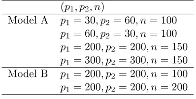
2-layered Network. To compare the proposed method with the most recent method-ology that also provides estimates for the regression parameters and the precision matrix (CAPME, Cai et al. (2012)), we use the exact same model settings that have been used in that paper. Specifically, we consider the following two models:
• Model A: Each entry inB∗ is nonzero with probability 5/p1, and off-diagonal entries for Θ∗ are nonzero with probability 5/p2.
• Model B: Each entry inB∗ is nonzero with probability 30/p1, and off-diagonal entries for Θ∗ are nonzero with probability 5/p2.
As in Cai et al.(2012), for both models, nonzero entries of B∗ and Θ∗ are generated from
Unif[(−1,−0.5)∪(0.5,1)], and diagonals of Θ∗ are set identical such that the condition number of Θ∗ isp2.
(p1, p2, n)
Model A p1= 30, p2 = 60, n= 100 p1= 60, p2 = 30, n= 100 p1= 200, p2= 200, n= 150 p1= 300, p2= 300, n= 150 Model B p1= 200, p2= 200, n= 100 p1= 200, p2= 200, n= 200
Table 1: Model Dimensions for Model A and B
To evaluate the selection performance of the algorithm, we use sensitivity (SEN), speci-ficity (SPE) and Mathews Correlation Coefficient (MCC) as criteria:
SEN = TN
TN + FP, SPE =
TP
TP + FN, MCC =
TP×TN−FP×FN
p
Further, to evaluate the accuracy of the magnitude of the estimates, we use the relative error in Frobenius norm:
rel-Fnorm = kBe−B
∗k
F
kB∗k
F
or kΘe−Θ
∗
kF
kΘ∗
kF .
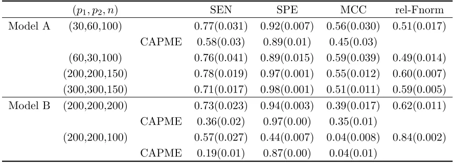
Tables 2 and 3 show the results for both the regression matrix and the precision matrix. For the precision matrix estimation, we compare our result with those available inCai et al. (2012), denoted as CAPME.
(p1, p2, n) SEN SPE MCC rel-Fnorm
Model A (30,60,100) 0.96(0.018) 0.99(0.004) 0.93(0.014) 0.22(0.029) (60,30,100) 0.99(0.009) 0.99(0.003) 0.93(0.017) 0.18(0.021) (200,200,150) 0.99(0.001) 0.99(0.001) 0.88(0.009) 0.18(.007) (300,300,150) 1.00(0.001) 0.99(0.001) 0.84(0.010) 0.21(0.007) Model B (200,200,200) 0.970(0.004) 0.982(0.001) 0.927(0.002) 0.194 (0.009)
(200,200,100) 0.32(0.010) 0.99(0.001) 0.49(0.009) 0.85(0.006)
Table 2: Performance evalution for the estimated regression matrix, over 50 replications
(p1, p2, n) SEN SPE MCC rel-Fnorm
Model A (30,60,100) 0.77(0.031) 0.92(0.007) 0.56(0.030) 0.51(0.017) CAPME 0.58(0.03) 0.89(0.01) 0.45(0.03)
(60,30,100) 0.76(0.041) 0.89(0.015) 0.59(0.039) 0.49(0.014) (200,200,150) 0.78(0.019) 0.97(0.001) 0.55(0.012) 0.60(0.007) (300,300,150) 0.71(0.017) 0.98(0.001) 0.51(0.011) 0.59(0.005) Model B (200,200,200) 0.73(0.023) 0.94(0.003) 0.39(0.017) 0.62(0.011)
CAPME 0.36(0.02) 0.97(0.00) 0.35(0.01)
(200,200,100) 0.57(0.027) 0.44(0.007) 0.04(0.008) 0.84(0.002) CAPME 0.19(0.01) 0.87(0.00) 0.04(0.01)
Table 3: Performance evaluation for estimated precision matrix, over 50 replications
As it can be seen from Tables 2 and 3, the sample size is a key factor that affects the performance. Our proposed algorithm performs extremely well in its selection properties onB and strikes a good balance between sensitivity and specificity in estimating Θ. 3 For
most settings, it provides substantial improvements over the CAPME estimator.
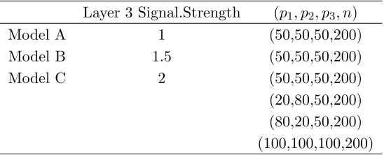
3-layer Network. For a 3-layer network, we consider the following data generation mechanism: for all three models A, B and C, each entry inBXY is nonzero with probability
3. In practice, for the debias Lasso procedure, we use the default choice of tuning parameters suggested in the implementation of the code provided in Javanmard and Montanari(2014); for FWER, we suggest usingα= 0.1 as the thresholding level; for tuning parameter selection, we suggest doing a grid search for (λn, ρn) on [0,0.5
p
logp1/n]×[0,0.5
p
5/p1, each entry inBXZ and BY Z is nonzero with probability 5/(p1+p2), and off-diagonal entries in Θ,Z are nonzero with probability 5/p3. Similar to the 2-layered set-up, the
nonzero entries in Θ,Z are generated from Unif[(−1,−0.5)∪(0.5,1)] with its diagnals set
identical such that its condition number is p3. For the regression matrices in the three models, nonzeros in BXY are generated from Unif[(−1,−0.5)∪(0.5,1)], and nonzeros in
BXZ andBY Z are generated from{Unif[(−1,−0.5)∪(0.5,1)]∗Signal.Strength}, where the
signal strength in the three models are given by 1, 1.5 and 2, respectively. More specifically, for Model A, B and C, nonzeros inBXZorBY Zare generated fromUnif[(−1,−0.5)∪(0.5,1)],
Unif[(−1.5,−0.75)∪(0.75,1.5)] and Unif[(−2,−1)∪(1,2)], respectively.
Layer 3 Signal.Strength (p1, p2, p3, n)
Model A 1 (50,50,50,200)
Model B 1.5 (50,50,50,200)
Model C 2 (50,50,50,200)
(20,80,50,200) (80,20,50,200) (100,100,100,200)
Table 4: Model Dimensions and Signal Strength for Model A, B and C
As mentioned in the beginning of this subsection, we only evaluate the algorithm’s performance onBXZ, BY Z and Θ,Z.
Based on the results shown in Tables 5, 6 and 7, the signal strength across layers affects the accuracy of the estimation, which is in accordance with what has been discussed regarding identifiability. Overall, the MLE estimator performs satisfactorily across a fairly wide range of settings and in many cases achieving very high values for the MCC criterion.
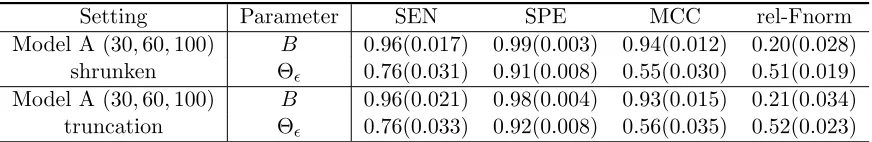
4.1.1 Simulation Results for non-Gaussian data
In many applications, the data may not be exactly Gaussian, but approximately Gaussian. Next, we present selected simulation results when the data comes from some distribution that deviates from Gaussian. Specifically, we consider two types of deviations based on the following transformations: (i) a truncated empirical cumulative distribution function and (ii) a shrunken empirical cumulative distribution functions as discussed in Zhao et al. (2015). In both simulation settings, we consider Model A with (p1, p2, n) = (30,60,100) under the two-layer setting, and the transformation is applied to errors in Layer 2. Table8 shows the simulation results for these two scenarios over 50 replications.
Based on the results in Table 8, relatively small deviations from the Gaussian distribu-tion do not affect the performance of the MLE estimates under the examined settings that are comparable to those obtained with Gaussian distributed data.
4.2 A comparison with the two-step estimator in Cai et al. (2012)
(p1, p2, p3, n) SEN SPE MCC rel-Fnorm Model A (50,50,50,200) 0.51(0.065) 0.99(0.001) 0.69(0.049) 0.68(0.050) Model B (50,50,50,200) 0.85(0.043) 0.99(0.001) 0.898(0.025) 0.36(0.056) Model C (50,50,50,200) 0.97(0.018) 0.99(0.002) 0.96(0.016) 0.16(0.040) (20,80,50,200) 0.55(0.078) 0.99(0.001) 0.72(0.059) 0.63(0.066) (80,20,50,200) 0.99(0.006) 0.99(0.002) 0.94(0.017) 0.076(0.032) (100,100,100,200) 1.00(0.001) 0.99(0.001) 0.87(0.016) 0.07(0.007)
Table 5: Performance evaluation for estimated regression matrixBXZ over 50 replications
(p1, p2, p3, n) SEN SPE MCC rel-Fnorm Model A (50,50,50,200) 0.53(0.051) 1.00(0.000) 0.72(0.036) 0.65(0.041) Model B (50,50,50,200) 0.90(0.033) 1.00(0.000) 0.95(0.019) 0.25(0.049) Model C (50,50,50,200) 0.98(0.013) 1.00(0.000) 0.99(0.007) 0.12(0.042) (20,80,50,200) 0.95(0.013) 1.00(0.000) 0.98(0.007) 0.19(0.030) (80,20,50,200) 0.96(0.027) 0.99(0.001) 0.97(0.022) 0.14(0.063) (100,100,100,200) 1.00(0.000) 1.00(0.000) 0.99(0.002) 0.025(0.002)
Table 6: Performance evaluation for estimated regression matrixBY Z over 50 replications
(p1, p2, p3, n) SEN SPE MCC rel-Fnorm
Model A (50,50,50,200) 0.69(0.044) 0.638(0.032) 0.20(0.036) 0.82(0.017) Model B (50,50,50,200) 0.77(0.050) 0.82(0.036) 0.42(0.071) 0.68(0.040) Model C (50,50,50,200) 0.88(0.041) 0.91(0.019) 0.63(0.059) 0.56(0.034) (20,80,50,200) 0.72(0.041) 0.80(0.028) 0.36(0.050) 0.72(0.021) (80,20,50,200) 0.90(0.028) 0.92(0.011) 0.68(0.039) 0.58(0.018) (100,100,100,200) 0.96(0.014) 0.96(0.003) 0.68(0.016) 0.049(0.010)
Table 7: Performance evaluation for estimated precision matrix Θ,Z over 50 replications
Setting Parameter SEN SPE MCC rel-Fnorm
Model A (30,60,100) B 0.96(0.017) 0.99(0.003) 0.94(0.012) 0.20(0.028) shrunken Θ 0.76(0.031) 0.91(0.008) 0.55(0.030) 0.51(0.019)
Model A (30,60,100) B 0.96(0.021) 0.98(0.004) 0.93(0.015) 0.21(0.034) truncation Θ 0.76(0.033) 0.92(0.008) 0.56(0.035) 0.52(0.023)
Table 8: Simulation results forB and Θ over 50 replications under npn transformation
afterward. For illustration purposes, we only show the results for a single realization under Model A with p1 = 30, p2 = 60, n = 100, although similar results were obtained in other simulation settings. Figure 2shows the value of the objective function as a function of the iteration under both initialization procedures, while Table 9 shows how the cardinality of the estimates changes over iterations for both initializers. It can be seen that the iterative MLE algorithm significantly improves the value of the objective function over the CAPME initialization and also that the set of directed and undirected edges stabilizes after a couple iterations.
Figure 2: Comparison between Cai’s estimate and our estimate
0 1 2 3 4 5 6 refit
Our initializer Bb(k) 275 275 275 275 275 275 275 275 b
Θ(k) 282 255 247 247 248 248 248 260
CAPME initializer Bb(k) 433 275 275 275 275 275 275 275 b
Θ(k) 979 267 250 249 249 248 248 260
Table 9: Change in cardinality over iterations forB and Θ