Two-way Fluid-Structure Interaction Simulation of a Micro Horizontal
Axis Wind Turbine
Yi-Bao Chen
1, Zhi-Kui Wang
2, Gwo-Chung Tsai
3,*1,2 Department of Electromechanical and Automobile Engineering, Yan Tai University, Yantai, China
3 Department of Mechanical and Electro-Mechanical Engineering,National I-Lan University, I-Lan, Taiwan, ROC.
Received 08 April 2014; received in revised form 27 December 2014; accepted 29 December 2014
Abstract
A two-way Fluid-Structure Interaction (FSI) analyses performed on a micro horizontal axis wind turbine
(HAWT) which coupled the CFX solver with Structural solver in ANSYS Workbench was conducted in this paper.
The partitioned approach-based non-conforming mesh methods and the k-ε turbulence model were adopted to
perform the study. Both the results of one-way and two-way FSI analyses were presented and compared with each
other, and discrepancy of the results, especially the mechanical properties, were analysed. Grid convergence which is
crucial to the results was performed, and the relationship between the inner flow field domain (rotational domain) and
the number of grids (number of cells, elements) was verified for the first time. Dynamical analyses of the wind turbine
were conducted using the torque as a reference value, to verify the rationality of the model which dominates the
accuracy of results. The optimal case was verified and used to conduct the study, thus, the results derived from the
simulation of the FSI are accurate and credible.
Keywords: fluid-structure interaction, flow field domain, dynamical analyses, grid convergence
1.
Introduction
Renewable Energy Sources (RES) plays a crucial role in modern electric systems because of its obvious advantages, such
as local availability, environment friendliness, and relative higher prices of fossil fuels as well as the development of
corresponding technology in using it. Wind turbines extract the wind power by the rotors from mechanical energy, and then
translate the mechanical energy into electrical power with the generator, achieving a relative widely utilization by these
machines. Small wind turbines can be categorized as micro (<1KW), mid-range (1KW-5KW) and mini wind turbines (>20KW)
[1]. The small wind turbines are the predominate wind power extracting devices in rural, suburban or even in the populated city
areas [2], where large scale wind turbines could not be installed due to space constraints and generation of noise. Micro wind
turbines, whose rated power is negligible when compared with large wind turbines, have some dramatic priorities, such as its
simple geometry structure with light weight, easy to mounted, lower purchase price, and less space constraints. These machines
rely solely on the torque produced by the wind acting on the blades to generate electrical power, rather than using the generator
as a motor to start and accelerate the rotor when the wind is strong enough to produce power [3].The torque produced by the
wind is vital to the wind turbine, thus, the study of aerodynamic properties on the wind turbine causing a growing body of
scholars. The FSI analyses takes full consideration of mechanical properties and aerodynamic properties of the wind turbine by
*Corresponding author. E-mail address: [email protected]
virtue of some relative numerical methods, such as conforming meshes methods and non-conforming methods.
The numerical procedures which were adopted to solve FSI problems can be broadly classified into two approaches: the
monolithic approach and the partitioned approach; this paper mainly focus on the partitioned approach. The partitioned
approach can be divided into one-way and two-way coupling [4].The fluid surface pressure acting at the surface of wind turbine
structure is transferred to the structure solver without any feedback from the structure solver to the fluid solver when using the
one-way FSI. In other words, the aerodynamic properties in vicinity of the wind turbine are not influenced by the solution in the
structural solver. However, the two-way FSI transfers the displacement of the structure to the fluid solver and create new fluid
mesh to accommodate the new interface location simultaneously. The two-way FSI can be achieved even several fluid and
structure computations are performed at every time step and used to integrate the equations for each domain [5]. Whereas, this
method is quite time-consuming as several computations are done at each time step. The FSI methods with conforming meshes
usually involve three fields: the fluid dynamics, structural dynamics and mesh movement [6]. Nicholls-Lee et al. [7] conducted
a full FSI analysis for a range of composites, bend-twist coupled blades on horizontal axis tidal turbines. The hydrodynamic
analysis of a vertical axis tidal turbine using the full FSI coupling scheme was implemented by Khalid et al. [8] to compare the
difference between the CFX independent simulations results and two-way FSI analyses results. Bazilevs et al. [9] and Hsu and
Bazilevs [10] employed the non-conforming interface discretization approach to conduct the FSI on the full scale wind turbine.
Grids which are called cells in CFD analyses are generally referred to the number of finite volumes divided in domains, which
play a significant role in the accuracy of results and efficiency of the solution to a large extent. Nabi and Al-Khoury [12] studied
the total grid number with only four cases to verify the best grid number to conduct their study, and Wang and Zhang [13]
conducted the grid convergence on a micro wind turbine to verify the finest total grid number with five cases. Obviously, few
cases were used to conduct the grid convergence as the simulation is time-consuming. To our best knowledge, none of these
studies have elaborated the relationship of grids number and flow field domain other than indicated a finest grid number for a
case.
In this paper, we conducted the two-way FSI analyses on a micro HAWT and compared the results with the one-way FSI
analyses. Dynamical analyses, which are critical to validate the rationality of a geometry model but few researches have paying
attention on this aspect, were conducted to verify the reasonability at first, then the grid convergence research was performed
with 20 cases. The relationship between the number of grids of flow field domain and wind turbine power was verified for the
first time.
2.
Wind Turbine Model
The micro HAWT is mainly consisted of five components: the blade, hub, tower, generator and tail. Materials for all these
components are given structural steel to conduct the study, and Table 1 shows details of this machine. Fig. 1(a) gives the original
geometry model of it, but a simplified model with some bolts, nuts and gaskets as well as three trestles removed from the
original model which is shown in Fig. 1(b) is used to conduct the FSI analyses. Though the model is simplified, key components
of it are preserved, and this can save a lot redundant computational time and achieve relative accurate results.
Table 1 Operational properties of the micro wind turbine
Rated Power Rated DC Voltage Rated Current Rated Speed Max Power Number of Blade
100 W DC 12V 8.8 A 860 RPM 115 W 3
Cut-in Wind
Speed Cut-out Wind Speed Security Wind Speed Rated Wind Speed
Rotor
Diameter Materials
(a) The original wind turbine model (b) The simplified wind turbine model Fig. 1 The micro horizontal axis wind turbine model
3.
CFD Simulations
3.1. Numerical Methods
The partitioned approach-based non-conforming mesh methods were adopted to conduct the FSI analyses of the micro
wind turbine. This approach treats the fluid and the structure as two computational fields which can be solved separately with
their respective mesh discretization and numerical algorithm [6]. The calculations for the fluid side which were used to solve the
Navier-Stokes equation is given by Eq. 1. The interfacial conditions where between the fluid and the structure using the explicit
solution procedure to exchange data interactively. The non-conforming mesh methods treat the boundary location and the
related interface conditions as constraints that imposed on the model equations [6]. Using these methods, the two-way FSI
solution becomes more accurate, especially for larger deflections in the structure that fluid field is strongly influenced by
structural deformation [14], and it can be a second-order time accuracy and more stable [5]. The k-ε turbulence model which is
a widely used two-equation turbulence model was also used in this study.
The k-ε turbulence model, where k is the turbulence kinetic energy and ε represents the turbulence eddy dissipation, is
given by Eq. (2)-(3) respectively.
v
v v p T f
t
(1)
where ν is the flow velocity, ρ is the fluid density, p is the pressure, T is the component of the total stress tensor, and ƒ represents
body forces.
( ) t
j k kb
j j k j
k k
U k P P
t x x x
(2)
1 2 1( )
( )
t
j k b
j j j
U C P C C P
t x x x k
Where k: turbulence kinetic energy per unit mass;
ɛ
: turbulence dissipation rate; Cɛ1: k-epsilon turbulence model constant,value :1.44; Cɛ2: k-epsilon turbulence model constant, value :1.92; Cu :k- turbulence model constant, value :0.09; Pk : shear
production of turbulence ; Uj: velocity magnitude ;
μ
: turbulence dissipation rate ;μ
t: turbulent viscosity ;ρ
: density;
σ
k:turbulence model constant for the k equation, value:1.0;
σ
ɛ: k- turbulence model constant, value :1.3; Pkb and Pɛb represent theinfluence of the buoyancy forces and details could be found in [11].
3.2. Design constraints
In order not to affect the accuracy of results in the CFD solver, a rational flow field domain which is consisted with a
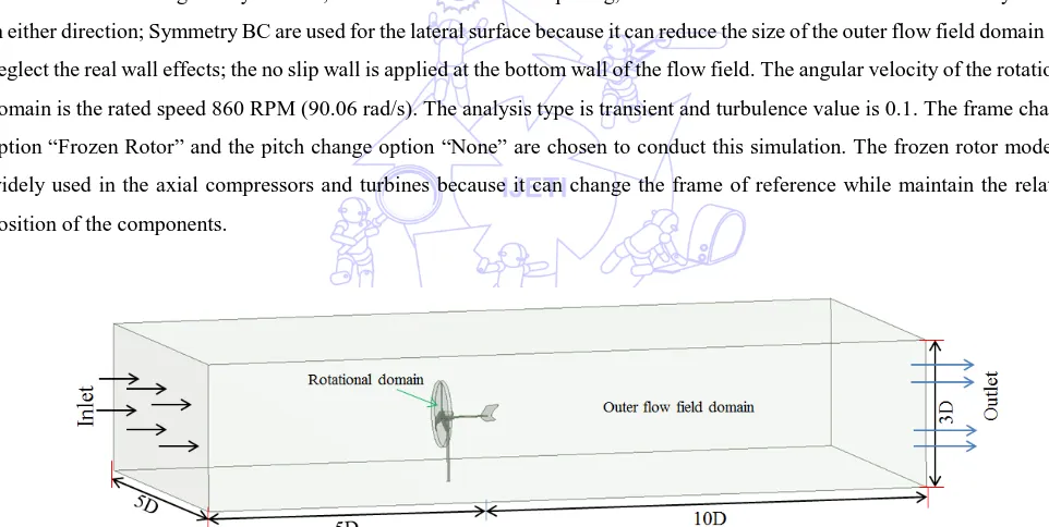
rotational flow field domain and outer flow field domain, causing much concerns on its grids number. Fig. 2 shows the flow field
domain which is used to conduct the FSI analyses in this study. The dimensions of the outer flow field domain, which is
multiples of the rotational domain’s diameters (D), have some differences in the upwind direction and downwind direction. The
outer flow field domain is extended to 5D in the upwind direction and 10D in the downwind direction. The dimension of the
downwind direction is longer than the upwind direction because the weak effects are taken into consideration. The other
dimensions at the inlet interface are 2.5D and 1.5D away from the canter of the rotational domain, respectively.
The boundary conditions (BC) of the flow field domain are defined as: the velocity value of the Inlet is the rated wind
speed 12m/s which is given by Table 1; the Outlet BC are set as opening, which allows the wind to cross the boundary surface
in either direction; Symmetry BC are used for the lateral surface because it can reduce the size of the outer flow field domain and
neglect the real wall effects; the no slip wall is applied at the bottom wall of the flow field. The angular velocity of the rotational
domain is the rated speed 860 RPM (90.06 rad/s). The analysis type is transient and turbulence value is 0.1. The frame change
option “Frozen Rotor” and the pitch change option “None” are chosen to conduct this simulation. The frozen rotor model is
widely used in the axial compressors and turbines because it can change the frame of reference while maintain the relative
position of the components.
Fig. 2 Boundary conditions and main dimensions of the computational domain
3.3. Dynamical Simulation
Dynamical simulation can simulate the operational manner of a model which is designed based on actual machines and
produce relative realistic results. The dynamical simulation of a model when used in a research with reasonable operating
conditions could give relatively accurate results to assess the rationality of a model and avoid errors caused by the geometry
model. However, few studies conducted on the FSI analyses of the wind turbine have paid attention to this aspect. We conducted
the dynamical simulation of the micro wind turbine with a dynamical module of the ANSYS Space Claim Design Modeller and
validated the rationality of the geometry model. The torque of the wind turbine is a critical factor as it has a direct relationship
with the wind turbine power; the centroid velocity of the wind turbine gives a better method to assess the kinetic characteristics
In Fig. 3, the centroid of the blade is denoted as a red point and the centroid trajectory which is a circle is highlighted in
light blue. The radius of the centroid trajectory is short for r (0.195m).
Fig. 3 Details of the model for the dynamical analyses
The total simulation time is 5s and the velocity of the wind turbine is 860 RPM. The rotational direction is clockwise and
the gravity is taken into consideration meanwhile. Fig. 4(a) and Fig. 4(b) show the dynamical properties of the micro wind
turbine clearly. Fig. 4(a) depicts that the maximum torque value occurs at the start up condition with a value nearly 1.114
Nm,and the torque sharply drops to a relative lower value with a value nearly 0.99 Nm. The torque fluctuates at the average
torque value 1.0042 Nm in such a little a range that it is negligible. Thus, we can conclude that the torque value of the micro
wind turbine is about 1 Nm. The torque value is relative smaller when compared with the rated value because some factors,
such as the air resistance, frictional resistance are not taken into consideration. As the torque value is fluctuating, thus it gives us
a hint that the centroid velocity of the blade should be varying with time as well. Fig. 4(b) shows that the centroid velocity of
each blade is varying with time. The centroid velocity of each blade though has a negligible difference between Blade_1 and
Blade_3 with a maximum difference nearly 0.002 m/s, which can be treated as a constant mean velocity value 17.623 m/s. The
theoretical value which is calculated with v = rω = 17.562 m/s, where r is the radius of the centroid trajectory (0.195m) and ω
is the rated speed 90.06 rad/s, has very little difference with the emulational value.
Fig. 4 Dynamical simulation properties of the micro HAWT
3.4. Grid Convergence
Grid convergence, which is also called the grid independence, plays a critical role in the accuracy and efficiency of the
computational simulation. Neither too much nor too less grids would satisfy the demand of efficiency and accuracy of the results.
Time (s)
0 1 2 3 4 5 6
T o rq u e ( N *m ) 0.96 0.98 1.00 1.02 1.04 1.06 1.08 1.10 1.12
Torque of the blades The maximum value Average torque value
(a) The emulational torque curve
Time (s)
0 1 2 3 4 5 6
V e lo c it y ( m /s ) 17.605 17.610 17.615 17.620 17.625 17.630 Blade_1_Velocity_Mag Blade_2_Velocity_Mag Blade_3_Velocity_Mag
Hou (et al. 2012) pointed out that in the FSI analyses, 80% of computational time is for the fluid, while only 10% for the
structure. As the size of grids in the computational fluid dynamics (CFD) solver is smaller than the structural solver, thus, it costs
more computational time. The outer flow field domain size is much larger than the rotational domain, therefore, a reasonable
grid density of the out flow field domain is crucial.
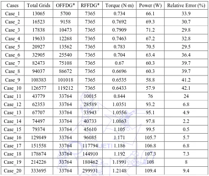
Table 2 Details of different cases and the wind turbine properties
*OFFDG: outer flow field domain grid; *RFFDG: rotational flow field domain
In this paper, 20 cases were divided to perform the grid convergence and the optimal case was determined and selected to
carry out the FSI analyses. Table 2 shows details of the number of cells and flow field domain. In Table 2, the torque and relative
error of each case are listed and elements number of each domain is given as well .The wind turbine power is a function of the
torque, which is given by Eq.(4).
9550 T n
P (4)
Where P is the electrical power; T is the torque of wind turbine, n is the rotational velocity. Thus, the rated torque calculated by
this equation is 1.11 Nm.
The relative error is written as
100% R R
R
P P
E P
(5)
Where ER represents the relative error; P and PR denote as the power calculated in these simulations and the rated power,
Cases Total Grids OFFDG* RFFDG* Torque (Nm) Power (W) Relative Error (%)
Case_1 13065 5700 7365 0.734 66.1 33.9
Case_2 16523 9158 7365 0.7692 69.3 30.7
Case_3 17838 10473 7365 0.7909 71.2 29.8
Case_4 19633 12268 7365 0.7463 67.2 32.8
Case_5 20927 13562 7365 0.783 70.5 29.5
Case_6 32905 25540 7365 0.704 63.4 36.4
Case_7 82473 75108 7365 0.67 60.3 39.7
Case_8 94037 86672 7365 0.6696 60.3 39.7
Case_9 108383 101018 7365 0.6535 58.8 41.2
Case_10 126577 119212 7365 0.6433 57.9 42.1
Case_11 43779 33764 10015 0.844 76 24
Case_12 62353 33764 28589 1.0351 93.2 6.8
Case_13 67707 33764 33943 1.0556 95.1 4.9
Case_14 74497 33764 40733 1.0863 97.8 2.2
Case_15 79374 33764 45610 1.105 99.5 0.5
Case_16 129849 33764 96085 1.171 105.7 5.7
Case_17 151558 33764 117794 1.186 106.8 6.8
Case_18 178674 33764 144910 1.192 107.3 7.3
Case_19 214226 33764 180462 1.1991 108 8
respectively.
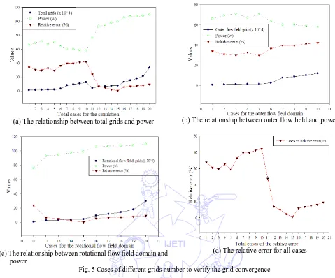
(a) The relationship between total grids and power (b) The relationship between outer flow field and power
(c) The relationship between rotational flow field domain and power
(d) The relative error for all cases
Fig. 5 Cases of different grids number to verify the grid convergence
We conducted the former 10 cases (case_1 to case_10) to figure out the significance of the out flow field domain grids
and another 10 cases to verify the rotational flow field domain grids. All these cases performed can be used to validate the
optimal case and analyze the relationship between grid number and accuracy as well as efficiency of results. The sizes of grid in
cases (case_1 to case_6) are coarse while case_7, case_8 and case_9 and case_10 have a better mesh. However, little difference
occurs when compared the torque among these cases. Though the number of total grids in case_10 is 9.67 times as big as the
case_1, however, the torque of the case_10 is smaller than case_1. It just elaborates that the relationship in these ten cases are
unpredictable. The optimal case is case_3, whose power is the maximum when compared with the rated power, that’s to say, this
case has the least error in these study. Thus, fewer grids can be used to conduct the FSI analyses because the accuracy of results
have indirect relationship with number of total cells. Considering that much computational time can be reduced with fewer grids,
an optimal case should be verified. The case_5 whose rotational flow field domain grids is used as a reference to validate the
effect of outer flow field domain grids on the results with another nine cases (from case_1 to case_10); and case_15, whose
relative error is 0.5% and the number of grids is reasonable, is used to verify the rotational flow field domain grids on the results
with cases (from case_11 to case_20). Finally, case_15 is chosen as the optimal to conduct this study.
Fig. 5(b) indicates the relationship between the outer flow field domain grids and power. It depicts that with the number
of grids from case_1 to case_10 are increasing, the power varying in the previous five cases while has an opposite relationship
results. Fig. 5(c) indicates that the tendency of the rotational flow field domain grids and the power achieves a good agreement.
Thus, we can conclude that the grid number of the rotational flow field domain dominates the accuracy of the FSI analytical
results.
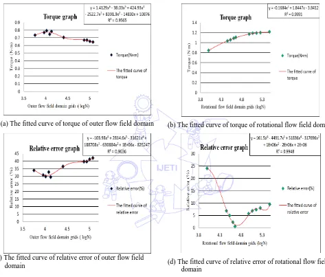
Figs. 5(b) and Fig. 5(c) depict the tendency of grids number and power clearly. However, the functional relationship with
the number of cells in flow field domain as the variable should be given to achieve a much more comprehensive cognition of it.
The fitted curve of torque and relative error are given using the Excel. As the relationship between torque and power is given
with Eq. 4, thus, the fitted curve of power is similar with torque.
(a) The fitted curve of torque of outer flow field domain (b) The fitted curve of torque of rotational flow field domain
(c) The fitted curve of relative error of outer flow field
domain (d) The fitted curve of relative error of rotational flow field
domain
Fig. 6 The fitted curves for different flow field domains
Considering the number of grids is relatively large, thus, logarithm is adopted to simplify the description. The fitted curve
y is located at the top right box and, the coefficient of determination R2 is the ratio of explained sum of squares (ESS) and total
sum of squares (TSS). The larger R2 the better fitted curve. Figs. 6(a) and Fig. 6(b) show the relationship of grids number and
power with different matched curves and R2. The fitted curve of the torque in Fig. 6(a) is a six order polynomial with
R2=0.9565; however, the fitted curve of torque can achieve the R2=0.991 with only two order polynomial. Thus, grids number
of the rotational flow field domain dominates the computational results. The fitted curve of relative error depicts the relationship
between grids number and relative error. The fitted curves in Figs. 6(c) and (d) are both six order polynomial, but the R2 of
rotational flow field domain is relatively larger than it for the outer flow field domain. Each of these two curves has a minimum
value point. However, the minimum value in Fig. 6(c) is 29.8% , which exceeds the rational ranges and in Fig. 6(d) is 0.5%,
4.
Results and Discussion
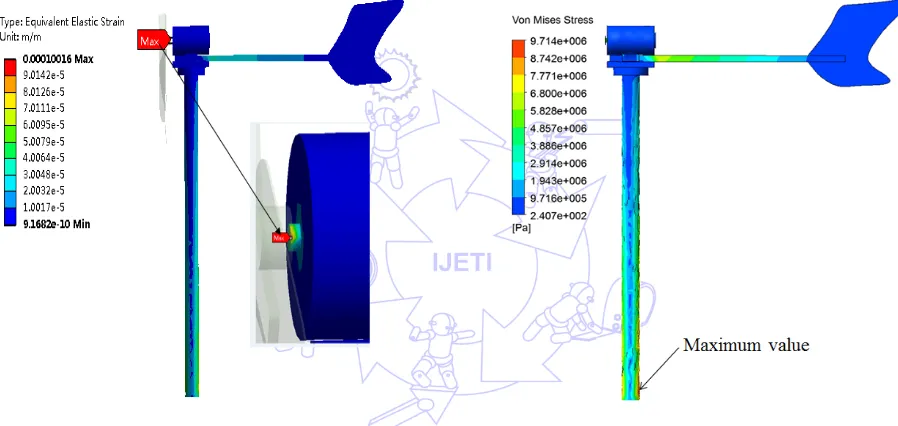
(a) The equivalent elastic strain of one-way FSI (b) The equivalent elastic strain of two-way FSI Fig. 7 A comparison of equivalent elastic strain using two different methods
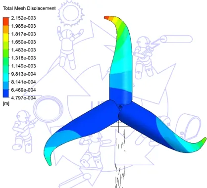
Fig. 8 The total mesh displacement of blade (two-way FSI)
Fig. 7 shows the results of equivalent elastic strain of the blades using one-way and two-way FSI analyses. Though the
mesh displacement is not taken into account in the one-way FSI analysis, which is shown in Fig. 7(a), differences in value of the
equivalent elastic strain is negligible when compared with two-way FSI. The position of the maximum value shown in these two
figures is consistent with each other and the maximum difference value of the equivalent elastic strain is within 1.07e-5, which
can be neglected in performing this study. Thus, both the one-way and two-way FSI analyses which is shown in Fig. 7(b) can
achieve an accurate result with a negligible change. It is primarily because that the rated wind speed causes little deformation of
the blades which are made of structural steel, thus, resulting in a negligible difference in these two methods.
The mesh displacement shown in Fig. 8 indicates that the maximum value occurs at the tip of the blade. The mesh
displacement is relatively smaller near the root of the blades. The mesh displacement can be a reflection of the deformation of
the blades because the new meshes are created to accommodate the interface location. Thus, we can affirm that the deformation
(a) The equivalent stress of one-way FSI
(b) The equivalent stress of two-way FSI
Fig. 9 A comparison of equivalent stress using two different methods
(a) The equivalent stress of other components of one-way FSI (a) The equivalent stress of other components of two-way FSI Fig. 10 A comparison of equivalent stress using two different methods
Distinguishing the priority between one-way and two-way FSI analyses seems impossible if we just conduct a
contradistinction of the equivalent elastic strain. Thus, the equivalent stress (von-Mises stress) of both the rotor and other
components were analyzed and compared with each other. Fig. 9(a) depicts the distribution of the equivalent stress on the rotor
in one-way FSI analyses. The position of the maximum von-Mises stress is not consistent with each other. The maximum
von-Mises value occurs at edge of the blade root in one-way FSI analysis, while the maximum von-Mises value shown in Fig.
9(b) occurs near the blade root. The von-Mises stress values in these two simulations have some difference while achieves a
good consistency with the position on blades with only little offset. Fig. 10 shows the distribution of equivalent stress of the
other components. The maximum stress value as well as the position have a dramatically difference. The maximum value of
stress 18.59 MPa in Fig. 10(a) occurs at the rotating shaft and in Fig. 10(b), the maximum value 9.71 MPa occurs at the location
near the bottom of the tower. The distribution of equivalent stress shown in Fig. 10(b) shows a reasonable result which is
5.
Conclusions
In this paper, the new designs of CCPGT have been generated in a systematic methodology. Firstly, the design
requirements and design constraints are summarized based on the characteristics of the existing CCPGT. Then, the atlas of new
designs are obtained through the process of the creative mechanism design approach, and 3 new designs synthesized from (5, 7)
graph have been obtained. Finally, the feasibility of the new designs is verified by conducting kinematic simulation. The result
has shown that the new designs can produce a more wide range of non-uniform output motion than the existing design, and are
better alternatives for driving a variable speed input mechanism.
(1) Dynamical simulation of the micro HAWT was performed and the results of torque and velocity were analyzed. The torque
demonstrated by the kinematic simulation presents a minor value by comparing with the rated torque and reasons were
explained. The torque and centroid velocity show a good agreement with the theoretical value, thus, the correctness of the
model can be achieved.
(2) Grid convergence was conducted and the optimal case was validated and used in this study. Grid convergence performed
with two flow field domain shows a good consistency between the power and the number of grids in the rotational flow
field domain. The relative error of the analyzed results was compared among cases and the best case was verified. Thus, the
accuracy and efficiency of the FSI analyses can be credible.
(3) The results derived from both the one-way and two-way FSI analyses were compared with each other and the accuracy of
the two-way FSI method was validated. The results, such as the stress and strain of the rotor, show a minor change in their
maximum value and position. However, distinctions occur in other components of the wind turbine. Thus, the two-way FSI
analyses have more credible results.
6.
Acknowledgements
The research is really thanked to Graduate Innovation Foundation of Yantai University (YJSZ201415), and the financial
support of the National Science Council, under Grants MOST 103-3113-E-002 -003.
References
[1]P. D. Clausen and D. H. Wood, "Research and development issues for small wind turbines," Renewable Energy, vol. 16.1, pp. 922-927, 1999.
[2]R. K. Singh and M. R. Ahmed, "Blade design and performance testing of a small wind turbine rotor for low wind speed
applications," Renewable Energy, vol. 50, pp. 812-819, 2013.
[3]A. K. Wright and D. H. Wood, "The starting and low wind speed behavior of a small horizontal axis wind turbine," Journal of Wind Engineering and Industrial Aerodynamics, vol. 92, pp. 1265-1279, 2004.
[4]F.-K. Benra, H. J. Dohmen, J. Pei, S. Schuster, and B. Wan, "A Comparison of One-Way and Two-Way Coupling Methods
for Numerical Analysis of Fluid-Structure Interactions," Journal of Applied Mathematics, vol. 2011, pp. 1-16, 2011. [5]V. Jean-Mark, D. Pascal, H. Charles & L. Benoit, "Strong coupling algorithm to solve fluid-structure interaction problems
with a staggered approach," Report, Open Engineering SA, 2009.
[6]G. Hou, J. Wang, and A. Layton, "Numerical Methods for Fluid-Structure Interaction - A Review," Communications in
Computational Physics, vol. 12, pp. 337-377, 2012.
[8]S. S. Khalid, Zhiguang, J., Fuding, T., Liang, Z., & Chaudhry, A. Z. , "CFD Simulation of Vertical Axis Tidal Turbine
Using Two-W ay Fluid Structure Interaction Method.pdf," In Applied Sciences and Technology, 10th International Bhurban Conference on. IEEE, pp. 286-291, 2013.
[9]Y. Bazilevs, M. C. Hsu, and M. A. Scott, "Isogeometric fluid–structure interaction analysis with emphasis on non-matching discretizations, and with application to wind turbines," Computer Methods in Applied Mechanics and Engineering, vol.
249-252, pp. 28-41, 2012.
[10] M.-C. Hsu and Y. Bazilevs, "Fluid–structure interaction modeling of wind turbines: simulating the full machine," Computational Mechanics, vol. 50, pp. 821-833, 2012.
[11] ANSYS, Inc, ANSYS Mechanical APDL Theory Reference, ANSYS, Inc, USA, 2012.
[12] M. Nabi and R. Al-Khoury, "An efficient finite volume model for shallow geothermal systems—Part II: Verification, validation and grid convergence," Computers & Geosciences, vol. 49, pp. 297-307, 2012.
[13] Y.-F. Wang and M.-S. Zhan, "3-Dimensional CFD simulation and analysis on performance of a micro-wind turbine resembling lotus in shape," Energy and Buildings, vol. 65, pp. 66-74, 2013.