Feature-Level Domain Adaptation
Wouter M. Kouw [email protected]
Laurens J.P. van der Maaten [email protected] Department of Intelligent Systems
Delft University of Technology
Mekelweg 4, 2628 CD , the Netherlands
Jesse H. Krijthe [email protected]
Department of Intelligent Systems Delft University of Technology
Mekelweg 4, 2628 CD Delft, the Netherlands Department of Molecular Epidemiology Leiden University Medical Center
Eindhovenweg 20, 2333 ZC Leiden, the Netherlands
Marco Loog [email protected]
Department of Intelligent Systems Delft University of Technology
Mekelweg 4, 2628 CD Delft, the Netherlands The Image Group,
University of Copenhagen
Universitetsparken 5, DK-2100, Copenhagen , Denmark
Editor:Urun Dogan, Marius Kloft, Francesco Orabona, and Tatiana Tommasi
Abstract
Domain adaptation is the supervised learning setting in which the training and test data are sampled from different distributions: training data is sampled from a source domain, whilst test data is sampled from a target domain. This paper proposes and studies an approach, called feature-level domain adaptation (flda), that models the dependence between the two domains by means of a feature-level transfer model that is trained to describe the transfer from source to target domain. Subsequently, we train a domain-adapted classifier by minimizing the expected loss under the resulting transfer model. For linear classifiers and a large family of loss functions and transfer models, this expected loss can be computed or approximated analytically, and minimized efficiently. Our empirical evaluation offlda focuses on problems comprising binary and count data in which the transfer can be naturally modeled via a dropout distribution, which allows the classifier to adapt to differences in the marginal probability of features in the source and the target domain. Our experiments on several real-world problems show thatfldaperforms on par with state-of-the-art domain-adaptation techniques.
1. Introduction
Domain adaptation is an important research topic in machine learning and pattern recogni-tion that has applicarecogni-tions in, among others, speech recognirecogni-tion (Leggetter and Woodland, 1995), medical image processing (Van Opbroek et al., 2013), computer vision (Saenko et al., 2010), social signal processing (Zen et al., 2014), natural language processing (Peddinti and Chintalapoodi, 2011), and bioinformatics (Borgwardt et al., 2006). Domain adaptation deals with supervised-learning settings in which the common assumption that the training and the test observations stem from the same distribution is dropped. This learning setting may arise, for instance, when the training data is collected with a different measurement device than the test data, or when a model that is trained on one data source is deployed on data that comes from another data source. This creates a learning setting in which the training set contains samples from one distribution (the so-called source domain), whilst the test set constitutes samples from another distribution (the target domain). In domain adaptation, one generally assumes a transductive learning setting: that is, it is assumed that the unlabeled test data are available to us at training time and that the main goal is to predict their labels as well as possible.
The goal of domain-adaptation approaches is to exploit information on the dissimilarity between the source and target domains that can be extracted from the available data in order to make more accurate predictions on samples from the target domain. To this end, many domain adaptation approaches construct asample-level transfer model that assigns weights to observations from the source domain in order the make the source distribution more similar to the target distribution (Shimodaira, 2000; Huang et al., 2006; Cortes et al., 2008; Gretton et al., 2009; Cortes and Mohri, 2011). In contrast to such sample-level reweighing approaches, in this work, we develop afeature-level transfer model that describes the shift between the target and the source domain for each feature individually. Such a feature-level approach may have advantages in certain problems: for instance, when one trains a natural language processing model on news articles (the source domain) and applies it to Twitter data (the target domain), the marginal distribution of some of the words or n-grams (the features) is likely to vary between target and source domain. This shift in the marginal distribution of the features cannot be modeled well by sample-level transfer models, but it can be modeled very naturally by a feature-level transfer model.
problems in which the features are binary or count data (as often encountered in natural language processing), but the approach we describe is more generally applicable. In addi-tion to experiments on artificial data, we present experiments on several real-world domain adaptation problems, which show that our feature-level approach performs on par with the current state-of-the-art in domain adaptation.
The outline of the remainder of this paper is as follows. In Section 2, we give an overview of related prior work on domain adaptation. Section 3 presents our feature-level domain adaptation (flda) approach. In Section 4, we present our empirical evaluation of
feature-level domain adaptation and Section 5 concludes the paper with a discussion of our results.
2. Related Work
Current approaches to domain adaptation can be divided into one of three main types. The first type constitutes importance weighting approaches that aim to reweigh samples from the source distribution in an attempt to match the target distribution as well as possible. The second type aresample transformationapproaches that aim to transform samples from the source distribution in order to make them more similar to samples from the target dis-tribution. The third type arefeature augmentationapproaches that aim to extract features that are shared across domains. Our feature-level domain adaptation (flda) approach is
an example of a sample-transformation approach.
2.1 Importance Weighting
Importance-weighting approaches assign a weight to each source sample in such a way as to make the reweighed version of the source distribution as similar to the target distribution as possible (Shimodaira, 2000; Huang et al., 2006; Cortes et al., 2008; Gretton et al., 2009; Cortes and Mohri, 2011; Gong et al., 2013; Baktashmotlagh et al., 2014). If the class pos-teriors are identical in both domains (that is, the covariate-shift assumption holds) and the importance weights are unbiased estimates of the ratio of the target density to the source density, then the importance-weighted classifier converges to the classifier that would have been learned on the target data if labels for that data were available (Shimodaira, 2000). De-spite their theoretic appeal, importance-weighting approaches generally do not to perform very well when the data set is small, or when there is little ”overlap” between the source and target domain. In such scenarios, only a very small set of samples from the source domain is assigned a large weight. As a result, the effective size of the training set on which the classifier is trained is very small, which leads to a poor classification model. In contrast to importance-weighting approaches, our approach performs afeature-levelreweighing. Specif-ically, flda assigns a data-dependent weight to each of the features that represents how
informative this feature is in the target domain. This approach effectively uses all the data in the source domain and therefore suffers less from the small sample size problem.
2.2 Sample Transformation
2011; Gong et al., 2012; Baktashmotlagh et al., 2013; Dinh et al., 2013; Fernando et al., 2013; Shao et al., 2014). Most sample-transformation approaches learn global (non)linear transformations that map source and target data points into the same, shared feature space in such a way as to maximize the overlap between the transformed source data and the transformed target data (Gopalan et al., 2011; Pan et al., 2011; Gong et al., 2012; Fernando et al., 2013; Baktashmotlagh et al., 2013). Approaches that learn a shared subspace in which both the source and the target data are embedded often minimize the maximum mean discrepancy (MMD) between the transformed source data and the transformed target data (Pan et al., 2011; Baktashmotlagh et al., 2013). If used in combination with a universal kernel, the MMD criterion is zero when all the moments of the (transformed) source and target distribution are identical. Most methods minimize the MMD subject to constraints that help to avoid trivial solutions (such as collapsing all data onto the same point) via some kind of spectral analysis. An alternative to the MMD is the subspace disagreement measure (SDM) of Gong et al. (2012), which measures the discrepancy of the angles between the principal components of the transformed source data and the transformed target data. Most current sample-transformation approaches work well for ”global” domain shifts such as translations or rotations in the feature space, but they are less effective when the domain shift is ”local” in the sense that it strongly nonlinear. Similar limitations apply to the
flda approach we explore, but it differs in that (1) our transfer model does not learn a
subspace but operates in the original feature space and (2) the measure it minimizes to model the transfer is different, namely, the negative log-likelihood of the target data under the transferred source distribution.
2.3 Feature Augmentation
Several domain-adaptation approaches extend the source data and the target data with additional features that are similar in both domains (Blitzer et al., 2006; Li et al., 2014). Specifically, the approach by Blitzer et al. (2006) tries to induce correspondences between the features in both domains by identifying so-called pivot features that appear frequently in both domains but that behave differently in each domain; SVD is applied on the resulting pivot features to obtain a low-dimensional, real-valued feature representation that is used to augment the original features. This approach works well for natural language processing problems due to the natural presence of correspondences between features, e.g. words that signal each other. The approach of Blitzer et al. (2006) is related to many of the instantiations of flda that we consider in this paper, but it is different in the sense that
we only use information on differences in feature presence between the source and the target domain to reweigh those features (that is, we do not explicitly augment the feature representation). Moreover, the formulation of flda is more general, and can be extended
through a relatively large family of transfer models.
3. Feature-Level Domain Adaptation
with a domain-adaptation problem on which the classifier trained on book reviews will likely not work very well: the classifier will assign large positive weights to, for instance, words such as ”interesting” and ”insightful” as these suggest positive book reviews and will be assigned large positive weights by a linear classifier. But these words hardly ever appear in reviews of kitchen appliances. As a result, a classifier trained naively on the book reviews may perform poorly on kitchen appliance reviews. Since the target domain data (the kitchen appliance reviews) are available at training time, a natural approach to resolving this problem may be to down-weigh features corresponding to words that do not appear in the target reviews, for instance, by applying a high level of dropout (Hinton et al., 2012) to the corresponding features in the source data when training the classifier. The use of dropout mimics the target domain scenario in which the ”interesting” and ”insightful” features are hardly ever observed during the training of the classifier, and prevents that these features are assigned large positive weights during training. Feature-level domain adaptation flda
aims to formalize this idea in a two-stage approach that (1) fits a probabilistic sample transformation model that aims to model the transfer between source and target domain and (2) trains a classifier by minimizing the risk of the source data under the transfer model. In the first stage, flda models the transfer between the source and the target domain:
the transfer model is a data-dependent distribution that models the likelihood of target data conditioned on observed source data. Examples of such transfer models may be a dropout distribution that assigns a likelihood of 1−θto the observed feature value in the source data and a likelihood ofθto a feature value of 0, or a Parzen density estimator in which the mean of each kernel is shifted by a particular value. The parameters of the transfer distribution are learned by maximizing the likelihood of target data under the transfer distribution (conditioned on the source data). In the second stage, we train a linear classifier to minimize the expected value of a classification loss under the transfer distribution. For quadratic and exponential loss functions, this expected value and its gradient can be analytically derived whenever the transfer distribution factorizes over features and is in the natural exponential family; for logistic and hinge losses, practical upper bounds and approximations can be derived (Van der Maaten et al., 2013; Wager et al., 2013; Chen et al., 2014).
In the experimental evaluation offlda, we focus on applying dropout transfer models to
domain-adaptation problems involving binary and count features. These features frequently appear in, for instance, bag-of-words features in natural language processing (Blei et al., 2003) or bag-of-visual-words features in computer vision (J´egou et al., 2012). However, we note that flda can be used in combination with a larger family of transfer models; in
particular, the expected loss that is minimized in the second stage offldacan be computed
or approximated efficiently for any transfer model that factorizes over variables and that is in the natural exponential family.
3.1 Notation
We assume a domain adaptation setting in which we receive pairs of samples and labels from thesourcedomain,S ={(xi, yi)|xi∼pX, yi∼pY | X,xi ∈Rm, yi ∈Y}|i=1S|, at training time.
time, we receive samples from thetarget domain,T ={zj|zj ∼pZ,zj ∈Rm}|j=1T| that need
to be classified. Note that we assume samples xi and zj to lie in the same m-dimensional feature spaceRm, hence, we assume that pX andpZ are distributions over the same space.
For brevity, we occasionally adopt the notation X=
x1, . . . ,x|S|
,Z=
z1, . . . ,z|T|
, and
y=y1, . . . , y|S|
.
3.2 Target Risk
We adopt an empirical risk minimization (ERM) framework for constructing our domain-adapted classifier. The ERM framework proposes a classification functionh:Rm →R and assesses the quality of the hypothesis by comparing its predictions with the true labels on the empirical data using a loss functionL:Y ×R→R+0. The empirical loss is an estimate
of the risk, which is defined as the expected value of the loss function under the data distribution. Below, we show that if the target domain carries no additional information about the label distribution, the risk of a model on the target domain is equivalent to the risk on the source domain under a particular transfer distribution.
We first note that the joint source data, target data and label distribution can be de-composed into two conditional distributions and one marginal source distribution;pY,Z,X =
pY | Z,X pZ | X pX. The first conditional pY | Z,X describes the full class-posterior
distribu-tion given both source and target distribudistribu-tion. Next, we introduce our main assumpdistribu-tion: the labels are conditionally independent of the target domain given the source domain (Y ⊥⊥ Z | X), which implies: pY | Z,X = pY | X. In other words, we assume that we can
construct an optimal target classifier if (1) we have access to infinitely many labeled source samples—we knowpY | X pX—and (2) we know the true domain transfer distributionpZ | X.
In this scenario, observing target labels yj ∼ pY | Z does not provide us with any new
information.
To illustrate our assumption, imagine a sentiment classification problem. If people frequently use the word ”nice” in positive reviews about electronics products (the source domain) and we know that electronics and kitchen products (the target domain) are very similar, then we assume that the word ”nice” is not predictive of negative reviews of kitchen appliances. In other words, knowing that ”nice” is predictive of a positive review and know-ing that the domains are similar, it cannot be the case that ”nice” is suddenly predictive of a negative review. Under this assumption, learning a good model for the target do-main amounts to transferring the source dodo-main to the target dodo-main (that is, altering the marginal probability of observing the word ”nice”) and learning a good predictive model on the resulting transferred source domain. Admittedly, there are scenarios in which our assumption is invalid: if people like ”small” electronics but dislike ”small” cars, the assump-tion is violated and our domain-adaptaassump-tion approach will likely work less well. We do note, however, that our assumption is less stringent than the covariate-shift assumption, which assumes that the posterior distribution over classes is identical in the source and the target domain (i.e. that pY | X =pY | Z): the covariate-shift assumption does not facilitate the use
Formally, we start by rewriting the risk RZ on the target domain as follows:
RZ(h) =
Z
Z
X
y∈Y
L(y, h(z))pY,Z(y,z) dz
= Z
Z
X
y∈Y
Z
X
L(y, h(z))pY,Z,X(y,z,x) dx dz
= Z
Z
X
y∈Y
Z
X
L(y, h(z))pY | Z,X(y|z,x) pZ | X(z|x) pX(x) dxdz.
Using the assumption pY | Z,X =pY | X (or equivalently, Y ⊥⊥ Z | X) introduced above, we
can rewrite this expression as:
RZ(h) =
Z
Z
X
y∈Y
Z
X
L(y, h(z))pY | X(y|x) pZ | X(z|x) pX(x) dxdz
= Z
Z
EY,X
L(y, h(z)) pZ|X(z|x)
dz.
Next, we replace the target riskRZ(h) with its empirical estimate ˆRZ(h|S) by plugging in
source dataS for the source joint distribution pY,X:
ˆ
RZ(h|S) =
1
|S|
Z
Z
X
(xi,yi)∈S
L(yi, h(z))pZ | X(z|x=xi) dz
= 1
|S|
X
(xi,yi)∈S
EZ | X=xi
L(yi, h(z))
. (1)
Feature-level domain adaptation (flda) trains classifiers by constructing a parametric
model of the transfer distribution pZ | X and, subsequently, minimizing the expected loss in
Equation 1 on the source data with respect to the parameters of the classifier. For linear classifiers, the expected loss in Equation 1 can be computed analytically for quadratic and exponential losses if the transfer distribution factorizes over dimensions and is in the natural exponential family; for the logistic and hinge losses, it can be upper-bounded or approximated efficiently under the same assumptions (Van der Maaten et al., 2013; Wager et al., 2013; Chen et al., 2014). Note that no observed target samples zj are involved
Equation 1; the expectation is over the transfer model pZ | X, conditioned on a particular
sample xi. The target data is only used to estimate the parameters of the transfer model.
3.3 Transfer Model
The transfer distribution pZ | X describes the relation between the source and the target
for a particular family of distributions. For instance, if we know that the main variation between two domains consists of particular words that are frequently used in one domain (say, news articles) but infrequently in another domain (say, tweets), then we choose a distribution that alters the relative frequency of words.
Given a model of the transfer distributionpZ | X and a model of the source distribution
pX, we can work out the marginal distribution over the target domain as
qZ(z|θ, η) =
Z
X
pZ | X(z|x, θ) pX(x|η) dx, (2)
whereθrepresents the parameters of the transfer model, andηthe parameters of the source model. We learn these parameters separately: first, we learnηby maximizing the likelihood of the source data under the modelpX(x|η) and, subsequently, we learnθ by maximizing
the likelihood of the target data under the compound model qZ(z|θ, η). Hence, we first
estimate the value of η by solving:
ˆ
η = arg max
η
X
xi∈T
logpX(xi|η).
Subsequently, we estimate the value of θby solving:
ˆ
θ= arg max
θ
X
zj∈T
logqZ(zj|θ,ηˆ). (3)
In this paper, we focus primarily on domain-adaptation problems involving binary and count features. In such problems, we wish to encode changes in the marginal likelihood of observing non-zero values in the transfer model. To this end, we employ a dropout distribution as transfer model that can model domain-shifts in which a feature occurs less often in the target domain than in the source domain. Learning a flda model with a
dropout transfer model has the effect of strongly regularizing weights on features that occur infrequently in the target domain.
3.3.1 Dropout Transfer
To define our transfer model for binary or count features, we first set up a model that describes the likelihood of observing non-zero features in the source data. This model comprises a product of independent Bernoulli distributions:
pX(xi|η) = m
Y
d=1
ηd1xid6=0 (1−ηd)1−1xid6=0, (4)
where1 is the indicator function andηd is the success probability (probability of non-zero
values) of feature d. For this model, the maximum likelihood estimate of ηd is simply the
sample average: ˆηd=|S|−1Pxi∈S1xid6=0.
unbiased dropout distribution (Wager et al., 2013; Rostamizadeh et al., 2011) that sets an observed feature in the source domain to zero in the target domain with probabilityθd:
pZ | X(z−d|x=xid, θd) =
(
θd ifz−d= 0
1−θd ifz−d=xid /(1−θd)
, (5)
where∀d: 0≤θd≤1, the subscript of z−d denotes the d-th feature for any target sample,
and where the outcome of not dropping out is scaled by a factor 1/(1−θd) in order to
center the dropout distribution on the particular source sample. We assume the transfer distribution factorizes over features to obtain: pZ | X(z|x=xi, θ) =
Qm
d pZ | X(z−d|x−d=
xid, θd). The equation above defines a transfer distribution for every source sample. We
obtain our final transfer model by sharing the parametersθbetween all transfer distributions and averaging over all source samples.
To compute the maximum likelihood estimate of θ, the dropout transfer model from Equation 5 and the source model from Equation 4 are plugged into Equation 2 to obtain (see Appendix A for details):
qZ(z|θ, η) = m
Y
d=1
Z
X
pZ | X(z−d|x−d, θd) pX(x−d|ηd) dx−d
=
m
Y
d=1
(1−θd)ηd
1z−d6=0
1−(1−θd) ηd
1−1z−d6=0
. (6)
Plugging this expression into Equation 3 and maximizing with respect to θ, we obtain:
ˆ
θd= max{0,1−
ˆ
ζd
ˆ
ηd },
where ˆζdis the sample average of the dichotomized target samples,|T|−1Pzj∈T 1zjd6=0, and
where ˆηd is the sample average of the dichotomized source samples, |S|−1Pxi∈S1xid6=0.
We note that our particular choice for the transfer model cannot represent rate changes in the values of non-zero count features, such as whether a word is used on average 10 times in a document versus used on average only 3 times. The only variation that our dropout distribution captures is the variation in whether or not a feature occurs (z−d6= 0).
Because our dropout transfer model factorizes over features and is in the natural expo-nential family, the expectation in Equation 1 can be analytically computed. In particular, for a transfer distribution conditioned on source samplexi, its mean and variance are:
EZ |xi
z =xi
VZ |xi
z
= diag θ 1−θ
◦xix>i ,
where◦denotes the element-wise product of two matrices and we use the shorthand notation EZ | X=xi =EZ |xi. The variance is a diagonal matrix due to our assumption of independent
3.4 Classification
In order to perform classification with the risk formulation in Equation 1, we need to select a loss function L. Popular choices for the loss function include the quadratic loss (used in least-squares classification), the exponential loss (used in boosting), the hinge loss (used in support vector machines) and the logistic loss (used in logistic regression). The formulation in (1) has been studied before in the context of dropout training for the quadratic, exponential, and logistic loss by Wager et al. (2013); Van der Maaten et al. (2013), and for hinge loss by Chen et al. (2014). In this paper, we focus on the quadratic and logistic loss functions, but we note that the flda approach can also be used in combination with
exponential and hinge losses.
3.4.1 Quadratic Loss
Assuming binary labels Y = {−1,+1}, a linear classifier h(z) = w>z parametrized by
w, and a quadratic loss function L = (y−w>z)2, the expectation in Equation 1 can be expressed as:
ˆ
RZ(w|S) =
X
(xi,yi)∈S
EZ |xi
(yi−w>z)2
= y>y−2w>EZ |X[Z]y>+w> EZ |X[Z]EZ |X[Z]>+VZ |X[Z]
w,
in which the data is augmented with 1 to capture the intercept, and in which we denote the (m+ 1)× |S|matrix of expectations asEZ | X=X[Z] =
h
EZ | X=x1[z], . . . , EZ | X=x|S|[z] i
and the (m+ 1)×(m+ 1) diagonal matrix of variances asVZ | X=X[Z] = P
xi∈SVZ | X=xi[z].
Deriving the gradient for this loss function and setting it to zero yields the following closed-form solution for the classifier weights:
w=
EZ |X[Z]EZ |X[Z]>+VZ |X[Z]
−1
EZ |X[Z]y>. (7)
In the case of a multi-class problem, i.e. Y ={1, . . . , K}, K predictors can be built in an one-vs-all fashion orK(K−1)/2 predictors in an one-vs-one fashion.
The solution in Equation 7 is very similar to the solution of a standard ridge regression model;w= XX>+λI−1Xy>. The main difference is that, in a standard ridge regressor, the regularization is independent of the data. By contrast, the regularization on the weights of thefldasolution is determined by the variance of the transfer model: hence, it is different
Algorithm 1 Binary fldawith dropout transfer model and quadratic loss function. procedure flda-q(S, T)
ford=1,. . . , m do
ˆ
ηd=|S|−1Pxi∈S1xid6=0
ˆ
ζd=|T|−1
P
zj∈T 1zjd6=0
θd= max
n
0,1−ζˆd /ηˆd
o
end for
w= XX>+ diag 1−θθ◦XX>−1Xy> . ◦Element-wise product
return sign(w>Z)
end procedure
3.4.2 Logistic Loss
Following the same choice of labels and hypothesis class as for the quadratic loss, the logistic version can be expressed as:
ˆ
RZ(w|S) =
1
|S|
X
(xi,yi)∈S
EZ |xi
−yiw>z+ log
X
y0∈Y
exp(y0w>z)
= 1
|S|
X
(xi,yi)∈S
−yiw>EZ |xi[z] +EZ |xi
log X
y0∈Y
exp(y0w>z)
. (8)
This is a convex function inwbecause the log-sum-exp of an affine function is convex, and because the expected value of a convex function is convex. However, the expectation cannot be computed analytically. Following Wager et al. (2013), we approximate the expectation of the log-partition function, A(w>z) = logP
y0∈Y exp(y0w>z), using a Taylor expansion
around the valueai=w>xi:
EZ |xi
A(w>z)
≈A(ai) +A0(ai)(EZ |xi[w
>z]−a i) +
1 2A
00(a
i)(EZ |xi[w
>z]−a i)2
= const +σ(−2w>xi)σ(2w>xi)w>VZ |xi[z]w, (9)
where σ(x) = 1/(1 + exp(−x)) is the sigmoid function. In the Taylor approximation, the first-order term disappears because we chose an unbiased transfer model: EZ |xi[w
>z] =
w>xi. The approximation cannot be minimized in closed-form: we repeatedly take steps in the direction of its gradient in order to minimize the approximation of the risk in Equation 8, as described in Algorithm 2 (see Appendix B for the gradient derivation). The algorithm can be readily extended to multi-class problems by replacing w by a (m+ 1)×K matrix and using an one-hot encoding for the labels (see Appendix C).
4. Experiments
In our experiments, we first study the empirical behavior offldaon artificial data for which
Algorithm 2 Binary fldawith dropout transfer model and logistic loss function. procedure flda-l(S, T)
ford=1,. . . , m do
ˆ
ηd=|S|−1Pxi∈S1xid6=0
ˆ
ζd=|T|−1
P
zj∈T 1zjd6=0
θd= max
n
0,1−ζˆd /ηˆd
o
end for w= arg min
w0
−P
(xi,yi)∈S
yiw>xi]
+ w0> P
(xi,yi)∈S
σ −2w>xi
σ 2w>xi
diag 1−θθ
xix>i
w0
return sign(w>Z)
end procedure
4.1 Artificial Data
We first investigate the behavior offldaon a problem in which the model assumptions are
satisfied. We create such a problem setting by first sampling a source domain data set from known class-conditional distributions. Subsequently, we construct a target domain data set by sampling additional source data and transforming it using a pre-defined (dropout) transfer model.
4.1.1 Adaptation under Correct Model Assumptions
We perform experiments in which the domain-adapted classifier estimates the transfer model and trains on the source data; we evaluate the quality of the resulting classifier by comparing it to an oracle classifier that was trained on the target data (that is, the classifier one would train if labels for the target data were available at training time).
In the first experiment, we generate binary features by drawing 100,000 samples from two bivariate Bernoulli distributions. The marginal distributions are
0.7 0.7
for class one and
0.3 0.3
for class two. The source data is transformed to the target data using a dropout transfer model with parameters θ= 0.5 0. This means that 50% of the values for feature 1 are set to 0 and the other values are scaled by 1/(1−0.5). For reference, two naive least-squares classifiers are trained, one on the labeled source data (s-ls) and one on
the labeled target data (t-ls), and compared to flda-q. s-ls achieves a misclassification
error of 0.40 while t-ls and flda-qachieve an error of 0.30. This experiment is repeated
for the same classifiers but with logistic losses: a source logistic classifier (s-lr), a target
logistic classifier (t-lr) and flda-l. In this experiment, s-lr again achieves an error of
0.40 andt-lrand flda-lan error of 0.30. Figure 1 shows the decision boundaries for the
quadratic loss classifiers on the left and the logistic loss classifiers on the right. The figure shows that for both loss functions, flda has completely adapted to be equivalent to the
target classifier in this artificial problem.
Feature 1
0 1 2 3
Feature 2
0 0.5
1
Quadratic loss
flda-q tls sls
Feature 1
0 1 2 3
Feature 2
0 0.5
1
Logistic loss
flda-l tlr slr
Figure 1: Scatter plots of the target domain. The data was generated by sampling from bi-variate Bernoulli class-conditional distributions and transformed using a dropout transfer. Red and blue dots show different classes. The lines are the decision boundaries found by the source classifier (s-ls/s-lr), the target classifier ( t-ls/t-lr) and the adapted classifier (left flda-q, right flda-l). Note that the
decision boundary offldalies on top of the decision boundary oft-ls/t-lr.
Feature 1
0 10 20 30
Feature 2
0 5 10
Quadratic loss
flda-q tls sls
Feature 1
0 5 10 15 20 25
Feature 2
0 2 4 6 8 10
12 Logistic loss
flda-l tlr
slr
Figure 2: Scatter plots of the target domain with decision boundaries of classifiers. The data was generated by sampling from bivariate Poisson class-conditional distributions and the decision boundaries were constructed using the source classifier (s-ls/ s-lr), the target classifier (t-ls/t-lr), and the adapted classifiers (left flda-q,
rightflda-l). Note that the decision boundary offldalies on top of the decision
boundary oft-ls/ t-lr.
and dropping out the values of feature 1 with a probability of 0.5. In this experiments-ls
achieves an error of 0.181 and t-ls/ flda-qachieve an error of 0.099, whiles-lrachieves
an error of 0.170 andt-lr /flda-lachieve an error of 0.084. Figure 2 shows the decision
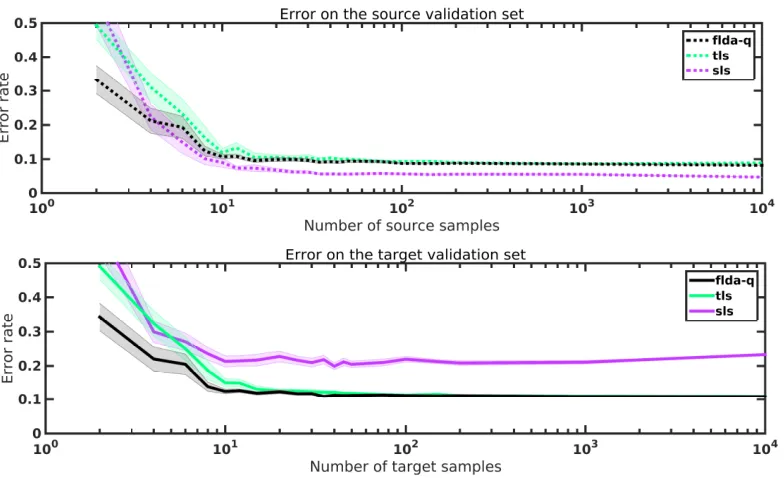
4.1.2 Learning Curves
One question that arises from the previous experiments is how many samplesfldaneeds to
estimate the transfer parameters and adapt to be (nearly) identical to the target classifier. To answer it, we performed an experiment in which we computed the classification error rate as a function of the number of training samples. The source training and validation data was generated from the same bivariate Poisson distributions as in Figure 2. The target data was constructed by generating additional source data and dropping out the first feature with a probability of 0.5. Each of the four data sets contained 10,000 samples. First, we trained a naive least-squares classifier on the source data (s-ls) and tested its performance
on both the source validation and the target sets as a function of the number of source training samples. Second, we trained a naive least-squares classifier on the labeled target data (t-ls) and tested it on the source validation and another target validation set as a
function of the number target training samples. Third, we trained an adapted classifier (flda-q) on equal amounts of labeled source training data and unlabeled target training
data and tested it on both the source validation and target validation sets. The experiment was repeated 50 times for every sample size to calculate the standard error of the mean.
The learning curves are plotted in Figure 3, which shows the classification error on the source validation set (top) and the classification error on the target validation (bottom). As expected, the source classifier (s-ls) outperforms the target (t-ls) and adapted (flda-q)
classifiers on the source domain (dotted lines), whileflda-q and t-lsoutperform s-lson
the target domain (solid lines). In this problem, it appears that roughly 20 labeled source samples and 20 unlabeled target samples are sufficient for flda to adapt to the domain
shift. Interestingly, flda-qis outperforming s-lsand t-lsfor small sample sizes. This is
most likely due to the fact that the application of the transfer model is acting as a kind of regularization. In particular, when the learning curves are computed with`2-regularized
classifiers, then the difference in performance disappears.
4.1.3 Robustness to Parameter Estimation Errors
Another question that arises is how sensitive the approach is to estimation errors in the transfer parameters. To answer this question, we performed an experiment in which we artificially introduce an error in the transfer parameters by perturbing them. As before, we generate 100,000 samples for both domains by sampling from bivariate Poisson distri-butions with λ=
2 2
for class 1 and λ= 6 6
for class 2. Again, the target domain is constructed by dropping out feature 1 with a probability of 0.5. We trained a naive classi-fier on the source data (s-ls), a naive classifier on the target data (t-ls), and an adapted
classifier flda-q with four different sets of parameters: the maximum likelihood estimate
of the first transfer parameter ˆθ1 with an addition of 0, 0.1, 0.2, and 0.3. Table 1 shows
Figure 3: Learning curves of the source classifier (s-ls), the target classifier (t-ls), and
adapted classifier (flda-q). The top figure shows the error on a validation set
generated from two bivariate Poisson distributions. The bottom figure shows the error on a validation set generated from two bivariate Poisson distributions with the first feature dropped out with a probability of 0.5.
sl tl θˆ1+ 0 θˆ1+ 0.1 θˆ1+ 0.2 θˆ1+ 0.3
Quadratic loss 0.245 0.137 0.138 0.145 0.149 0.150
Logistic loss 0.264 0.139 0.139 0.140 0.142 0.146
Table 1: Classification errors for a naive source classifier, a naive target classifier, and the adapted classifier with a value of 0, 0.1, 0.2, and 0.3 added to the estimate of the first transfer parameter ˆθ1.
transfer parameters to obtain high-quality adaptation. Nonetheless, our results do suggest thatflda is robust to relatively small perturbations.
4.2 Natural Data
In a second set of experiments, we evaluate flda on a series of real-world data sets and
Feature 1
0 5 10 15 20 25 30
Feature 2
0 5 10
Quadratic loss
flda-q0 flda-q1 flda-q2 flda-q3 sls tls
Feature 1
0 5 10 15 20 25 30
Feature 2
0 5 10
Logistic loss
flda-l0 flda-l1 flda-l2 flda-l3 slr tlr
Figure 4: Scatter plots of the target data and decision boundaries of two naive and four adapted classifiers with transfer parameter estimate errors of 0, 0.1, 0.2, and 0.3. Results are show for both the quadratic loss classifier (flda-q; left) and the
logistic loss classifier (flda-l; right).
As baselines, we consider eight alternative methods for domain adaptation. All of these employ a two-stage procedure. In the first step, sample weights, domain-invariant features, or a transformation of the feature space is estimated. In the second step, a classifier is trained using the results of the first stage. In all experiments, we estimate the hyperparam-eters, such as`2-regularization parameters, via cross-validation on held-out source data. It
should be noted that these values are optimal for generalizing to new source data but not necessarily for generalizing to the target domain (Sugiyama et al., 2007). Each of the eight baseline methods is described briefly below.
4.2.1 Naive Support Vector Machine (s-svm)
Our first baseline method is a support vector machine trained on only the source samples and applied on the target samples. We made use of the libsvm package by Chang and Lin (2011) with a radial basis function kernel and we performed cross-validation to estimate the kernel bandwidth and the`2-regularization parameter. All multi-class classification is done
through an one-vs-one scheme. This method can be readily compared to subspace align-ment (sa) and transfer component analysis (tca) to evaluate the effects of the respective
adaptation approaches.
4.2.2 Naive Logistic Regression (s-lr)
Our second baseline method is an`2-regularized logistic regressor trained on only the source
samples. Its main difference with the support vector machine is that it uses a linear model, a logistic loss instead of a hinge loss, and that it has a natural extension to multi-class as op-posed to one-vs-one. The value of the regularization parameter was set via cross-validation. This method can be readily compared to kernel mean matching (kmm), structural
cor-respondence learning (scl), as well as to the logistic loss version of feature-level domain
4.2.3 Kernel Mean Matching (kmm)
Kernel mean matching (Huang et al., 2006; Gretton et al., 2009) finds importance weights by minimizing the maximum mean discrepancy (MMD) between the reweighed source samples and the target samples. To evaluate the empirical MMD, we used the radial basis function kernel. The weights are then incorporated in an importance weighted`2-regularized logistic
regressor.
4.2.4 Structural Correspondence Learning (scl)
In order to build the domain-invariant subspace (Blitzer et al., 2006), the 20 features with the largest proportion of non-zero values in both domains are selected as the pivot features. Their values were dichotomized (1 if x 6= 0, 0 if x = 0) and predicted using a modified Huber loss (Ando and Zhang, 2005). The resulting classifier weight matrix was subjected to an eigenvalue decomposition and the eigenvectors with the 15 largest eigenvalues are retained. The source and target samples are both projected onto this basis and the resulting subspaces are added as features to the original source and target feature spaces, respectively. Consequently, classification is done by training an `2-regularized logistic regressor on the
augmented source samples and testing on the augmented target samples.
4.2.5 Transfer Component Analysis (tca)
For transfer component analysis, the closed-form solution to the parametric kernel map described in Pan et al. (2011) is computed using a radial basis function kernel. Its hyperpa-rameters (kernel bandwidth, number of retained components and trade-off parameterµ) are estimated through cross-validation. After mapping the data onto the transfer components, we trained a support vector machine with an RBF kernel, cross-validating over its kernel bandwidth and the regularization parameter.
4.2.6 Geodesic Flow Kernel (gfk)
The geodesic flow kernel is extracted based on the difference in angles between the principal components of the source and target samples (Gong et al., 2012). The basis functions of this kernel implicitly map the data onto all possible subspaces on the geodesic path between domains. Classification is performed using a kernel 1-nearest neighbor classifier. We used the subspace disagreement measure (SDM) to select an optimal value for the subspace dimensionality.
4.2.7 Subspace Alignment (sa)
hepat. ozone heart mam. auto. arrhy.
Features 19 72 13 4 24 279
Samples 155 2534 704 961 205 452
Classes 2 2 2 2 6 13
Missing 75 685 615 130 72 384
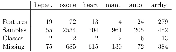
Table 2: Summary statistics of the UCI repository data sets with missing data.
4.2.8 Target Logistic Regression (t-lr)
Finally, we trained a `2-regularized logistic regressor using the normally unknown target
labels as the oracle solution. This classifier is included to obtain an upper bound on the performance of our classifiers.
4.2.9 Missing Data at Test Time
In this set of experiments, we study ”missing data at test time” problems in which we argue that dropout transfer occurs naturally. Suppose that for the purposes of building a classifier, a data set is neatly collected with all features measured for all samples. At test time, however, some features could not be measured, due to for instance sensor failure, and the missing values are replaced by 0. This setting can be interpreted as two distributions over the same space with their transfer characterized by a relative increase in the number of 0 values, which ourfldawith dropout transfer is perfectly suited for. We have collected
six data sets from the UCI machine learning repository (Lichman, 2013) with missing data: Hepatitis (hepat.), Ozone (ozone; Zhang and Fan, 2008), Heart Disease (heart; Detrano et al., 1989), Mammographic masses (mam.; Elter et al., 2007), Automobile (auto), and Arrhythmia (arrhy.; Guvenir et al., 1997). Table 2 shows summary statistics for these sets. In the experiments, we construct the training set (source domain) by selecting all samples with no missing data, with the remainder as the test set (target domain). We note that instead of doing 0-imputation, we also could have used methods such as mean-imputation (Rubin, 1976; Little and Rubin, 2014). It is worth noting that the flda framework can
adapt to such a setting by simply defining a different transfer model (one that replaces a feature value by its mean instead of a 0).
Table 3 reports the classification error rate of all domain-adaptation methods on the before-mentioned data sets. The lowest error rates for a particular data set are bold-faced. From the results presented in the table, we observe that whilst there appears to be little difference between the domains in the Hepatitis and Ozone data sets, there is substantial domain shift in the other data sets: the naive classifiers even perform at chance level on the Arrhythmia and Automobile data sets. On almost all data sets, both flda-qand flda-l
improve substantially over the s-lr, which suggests that they are successfully adapting to
s-svm s-lr kmm scl sa gfk tca flda-q flda-l t-lr
hepat. .213 .493 .347 .480 .253 .227 .213 .227 .200 .150
ozone .060 .124 .126 .136 .047 .093 .140 .047 .079 .069
heart .409 .338 .390 .319 .596 .362 .391 .203 .203 .177
mam. .331 .462 .446 .462 .323 .423 .323 .462 .431 .194
auto. .848 .935 .913 .935 .587 .565 .848 .848 .848 .371
arrhy. .930 .854 .620 .818 .414 .651 .930 .456 .889 .353
Table 3: Classification error rates on 6 UCI data sets with missing data. The data sets were partitioned into a training set (source domain), containing all samples with no missing features, and a test set (target domain), containing all samples with missing features.
4.2.10 Handwritten Digits
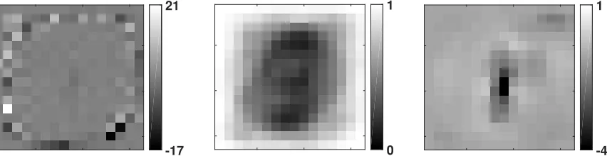
Handwritten digit data sets have been popular in machine learning due to the large sample size and the interpretability of the images. Generally, the data is acquired by assigning an integer value between 0 and 255 proportional to the amount of pressure that is applied at a particular spatial location on an electronic writing pad. Therefore, the probability of a non-zero value of a pixel informs us how often a pixel is part of a particular digit. For instance, the middle pixel in the digit 8 is a very important part of the digit because it nearly always corresponds to a high-pressure location, but the upper-left corner pixel is not used that often and is less important. Domain shift may be present between digit data sets due to differences in recording conditions. As a result, we may observe pixels that are discriminative in one data set (the source domain) that are hardly ever observed in another data set (the target domain). As a result, these pixels cannot be used to classify digits in the target domain, and we would like to inform the classifier that it should not assign a large weight to such pixels. We created a domain adaptation setting by considering two handwritten digit sets, namely MNIST (LeCun et al., 1998) and USPS (Hull, 1994). In order to create a common feature space, images from both data sets are resized to 16 by 16 pixels. To reduce the discrepancy between the size of MNIST data set (which contains 70,000 examples) and the USPS data set (which contains 9,298 examples), we only use 14,000 samples from the MNIST data set. The classes are balanced in both data sets.
Figure 5 shows a visualization of the probability that each pixel is non-zero for both data sets. The visualization shows that while the digits in the MNIST data set occupy mostly the center region, the USPS digits tend to occupy a substantially larger part of the image, specifically a center column. Figure 6 (left) visualizes the weights of the naive linear classifier (s-lr), (middle) the dropout probabilities θ, and (right) the adapted classifiers
weights (flda-l). The middle image shows that dropout probabilities are large in regions
xx 0
1
xx 0
1
Figure 5: Visualization of the probability of non-zero values for each pixel on the MNIST data set (left) and the USPS data set (right).
xx
xx -17
21
xx
xx 0
1
xx
xx -4
1
Figure 6: Weights assigned by the naive source classifier to the 0-digit predictor (left), the transfer parameters of the dropout transfer model (middle), and the weights assigned by the adapted classifier to the 0-digit predictor for training on USPS images and testing on MNIST (right;U →M).
smoothed in the periphery, which indicates that the classifier is placing more value on the center pixels and is essentially ignoring the peripheral ones.
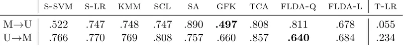
Table 4 shows the classification error rates where the rows correspond to the combi-nations of treating one data set as the source domain and the other as the target. The results show that there is a large difference between the domain-specific classifiers (s-lr
and t-lr), which indicates that the domains are highly dissimilar. We note that the error
rates of the target classifier on the MNIST data set are higher than usual for this data set (t-lr has an error rate of 0.234), which is because of the down-sampling of the images to
16×16 pixels and the smaller sample size. The results presented in the table highlight an interesting property offldawith dropout transfer: while fldaperforms well in settings in
s-svm s-lr kmm scl sa gfk tca flda-q flda-l t-lr
M→U .522 .747 .748 .747 .890 .497 .808 .811 .678 .055
U→M .766 .770 769 .808 .757 .660 .857 .640 .684 .234
Table 4: Classification error rates obtained on both combinations of treating one domain as the source and the other as the target. M=’MNIST’ and U=’USPS’.
s-svm s-lr kmm scl sa gfk tca flda-q flda-l t-lr
A→D .599 .618 .616 .621 .627 .624 .624 .599 .624 .303
A→W .688 .675 .668 .686 .606 .631 .712 .648 .678 .181
A→C .557 .553 .563 .555 .594 .614 .579 .565 .550 .427
D→W .312 .312 .346 .317 .167 .153 .295 .322 .312 .181
D→C .744 .712 .734 .712 .655 .706 .680 .712 .710 .427
W→C .721 .698 .709 .705 .677 .697 .688 .675 .701 .427
D→A .876 .719 .727 .724 .616 .680 .650 .700 .722 .258
W→A .676 .695 .706 .707 .631 .665 .668 .671 .691 .258
C→A .493 .523 .515 .496 .538 .592 .504 .490 .475 .258
W→D .198 .191 .178 .198 .214 .121 .166 .191 .185 .303
C→D .612 .616 .631 .583 .575 .599 .612 .510 .599 .303
C→W .712 .725 .729 .724 .600 .603 .695 .654 .702 .181
Table 5: Classification error rates obtained by ten (domain-adapted) classifiers for all pair-wise combinations of domains on the Office-Caltech data set with SURF features (A=’Amazon’, D=’DSLR’, W=’Webcam’, and C=’Caltech’).
4.2.11 Office-Caltech
The Office-Caltech data set (Hoffman et al., 2013) consists of images of objects gathered using four different methods: one from images found through a web image search (referred to as ’C’), one from images of products on Amazon (A), one taken with a digital SLR camera (D) and one taken with a webcam (W). Overall, the set contains 10 classes, with 1123 samples from Caltech, 958 samples from Amazon, 157 samples from the DSLR camera, and 295 samples from the webcam. Our first experiment with the Office-Caltech data set is based on features extracted through SURF features (Bay et al., 2006). These descriptors determine a set of interest points by finding local maxima in the determinant of the image Hessian. Weighted sums of Haar features are computed in multiple sub-windows at various scales around each of the interest points. The resulting descriptors are vector-quantized to produce a bag-of-visual-words histogram of the image that is both scale and rotation-invariant. We perform domain-adaptation experiments by training on one domain and testing on another.
Table 5 shows the results of the classification experiments, where compared to competing methods, sa is performing well for a number of domain pairs, which may indicate that
s-svm s-lr kmm scl sa gfk tca flda-q flda-l t-lr
A→D .406 .388 .402 .422 .460 .424 .351 .428 .388 .104
A→W .434 .468 .455 .474 .499 .477 .426 .491 .468 .064
D→W .086 .079 .083 .074 .103 .073 .087 .088 .079 .064
D→A .516 .496 .502 .497 .520 .569 .489 .589 .487 .216
W→A .520 .496 .514 .506 .541 .584 .510 .645 .501 .216
W→D .034 .030 .032 .034 .062 .052 .042 .024 .044 .104
Table 6: Classification error rates obtained by ten (domain-adapted) classifiers for all pairwise combinations of domains on the Office data set with DeCAF8 features
(A=’Amazon’, D=’DSLR’, and W=’Webcam’).
captured by subspace transformations. This result is further supported by the fact that the transformations found by gfk and tca are also outperforming s-svm. flda-q and flda-l are among the best performers on certain domain pairs. In general, flda does
appear to perform at least as good or better than a naive s-lr classifier. The results
on the Office-Caltech data set depend on the type of information the SURF descriptors are extracting from the images. We also studied the performance of domain-adaptation methods on a richer visual representation, produced by a pre-trained convolutional neural network. Specifically, we used a data set provided by Donahue et al., 2014, who extracted 1000-dimensional feature-layer activations (so-called DeCAF8 features) in the upper layers
of the a convolutional network that was pre-trained on the Imagenet data set. Donahue et al. (2014) used a larger superset of the Office-Caltech data set that contains 31 classes with 2817 images from Amazon, 498 from the DSLR camera, and 795 from the webcam. The results of our experiments with the DeCAF8 features are presented in Table 6. The
results show substantially lower error rates overall, but they also show that domain transfer in the the DeCAF8feature representation is not amenable to effective modeling by subspace
transformations. kmmandsclobtain performances that are similar to the of the naives-lr
classifier but in one experiment, the naive classifier is actually the best-performing model. Whilst achieving the best performance on 2 out of 6 domain pairs, theflda-qandflda-l
models are not as effective as on other data sets, presumably, because dropout is not a good model for the transfer in a continuous feature space such as the DeCAF8 feature space. 4.2.12 IMDb
bad only her she even film could time ever some
Proportion
non-zero values
0 0.1 0.2 0.3 0.4 0.5 0.6
Action Family War
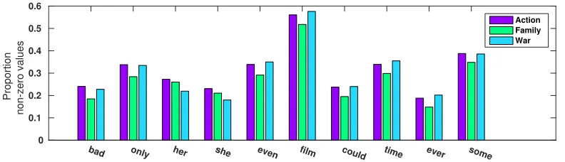
Figure 7: Proportion of non-zero values for a subset of words per domain on the IMDb data set.
s-svm s-lr kmm scl sa gfk tca flda-q flda-l t-lr
A→F .145 .136 .133 .133 .184 .276 .230 .135 .136 .196
A→W .158 .155 .155 .165 .163 .249 .266 .158 .154 .163
F→W .256 .206 .208 .206 .182 .289 .355 .205 .202 .163
F→A .201 .195 .193 .198 .193 .296 .363 .194 .194 .169
W→A .168 .160 .159 .159 .167 .238 .222 .155 .157 .169
W→F .340 .167 .163 .163 .232 .292 .203 .172 .159 .196
Table 7: Classification error rates obtained by ten (domain-adapted) classifiers for all pair-wise combinations of domains on the IMDb data set. (A=’Action’, F=’Family’, and W=’War’).
valid, we plot the proportion of non-zero values of 10 randomly chosen words per domain in Figure 7. The figure suggests that action movie and war movie reviews are quite similar, but the word use in family movie reviews does appear to be different.
Table 7 reports the results of the classification experiments on the IMDb database. The first thing to note is that the performances of s-lrand t-lr are quite similar, which
suggests that the frequencies of discriminative words do not vary too much between genres. The results also show that gfkand tca are not as effective on this data set as they were on the handwritten digits and Office-Caltech data sets, which suggests that finding a joint subspace that is still discriminative is hard, presumably, because only a small number of the 4180 words actually carry discriminative information. flda-q and flda-l are better suited for such a scenario, which is reflected by their competitive performance on all domain pairs.
4.2.13 Spam
wan cos cant msg dun meeting change interest million must looking
Proportion
non-zero values
0 0.02 0.04
0.06 sms
Figure 8: Proportion of non-zero values for a subset of words per domain on the spam data set.
s-svm s-lr kmm scl sa gfk tca flda-q flda-l t-lr
S→M .460 .522 .521 .524 .445 .491 .508 .511 .521 .073
M→S .830 .804 .799 .804 .408 .696 .863 .636 .727 .133
Table 8: Classification error rates obtained by ten (domain-adapted) classifiers for both domain pairs on the spam data set. (S=’SMS’ and M=’E-Mail’).
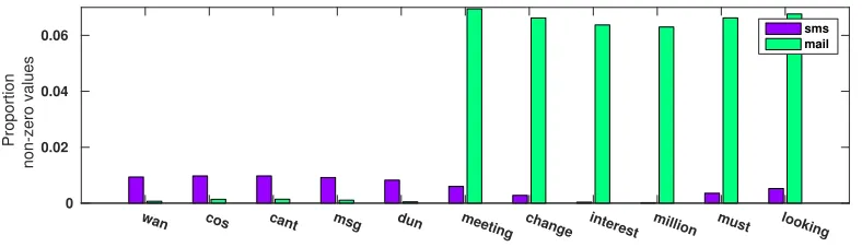
bag-of-words vectors over 4272 words that occurred in both data sets. Figure 8 shows the proportions of non-zero values for some example words, and shows that there exist large differences in word frequencies between the two domains. In particular, much of the domain differences are due to text messages using shortened words, whereas email messages tend to be more formal.
Table 8 shows results from our classification experiments on the spam data set. As can be seen from the results oft-lr, fairly good accuracies can be obtained on the spam detection
task. However, the domains are so different that the naive classifiers s-svm and s-lr are
performing according to chance or worse. Most of the domain-adaptation models do not appear to improve much over the naive models. Forkmmthis makes sense, as the importance
weight estimator will assign equal values to each sample when the empirical supports of the two domains are disjoint. There might be some features that are shared between domains, i.e., words that are spam in both emails and text messages, but considering the performance of sclthese might not be corresponding well with the other features. flda-qand flda-l
are showing slight improvements over the naive classifiers, but the transfer model we used is too poor as the domains contain a large amount of increased word frequencies.
4.2.14 Amazon
portrayed random indifferencebarbaric warming teens breath quality recipe waiting
Proportion
non-zero values
0 0.1 0.2 0.3 0.4 0.5
books dvds electronics kitchen
Figure 9: Proportion of non-zero values for a subset of words per domain on the Amazon data set.
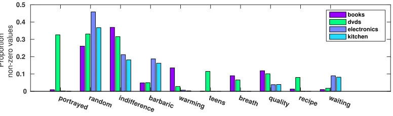
kitchen appliances (7945 reviews). Figure 9 shows the probability of a non-zero value for some example words in each category. Some words, such as ’portrayed’ or ’barbaric’, are very specific to one or two domains, but the frequencies of many other words do not vary much between domains. We performed experiments on the Amazon data set using the same experimental setup as before.
In Table 9, we report the classification error rates on all pairwise combinations of do-mains. The difference in classification errors between s-lr and t-lr is up to 10%, which
suggests there is potential for success with domain adaptation. However, the domain trans-fer is not captured well bysa,gfk,tca: on average, these methods are performing worse
than the naive classifiers. We presume this happens because only a small number of words are actually discriminative, and these words carry little weight in the sample transforma-tion measures used. Furthermore, there are significantly less samples than features in each domain which means models with large amounts of parameters are likely to experience estimation errors. By contrast, flda-lperforms strongly on the Amazon data set,
achiev-ing the best performance on many of the domain pairs. flda-q performs substantially
worse than flda-l, presumably, because of the singular covariance matrix and the fact
that least-squares classifiers are very sensitive to outliers.
5. Discussion and Conclusions
We have presented an approach to domain adaptation, calledflda, that fits a probabilistic
model to capture the transfer between the source and the target data and, subsequently, trains a classifier by minimizing the expected loss on the source data under this transfer model. Whilst the flda approach is very general, in this paper, we have focused on one
particular transfer model, namely, a dropout model. Our extensive experimental evaluation with this transfer model shows thatfldaperforms on par with the current state-of-the-art
methods for domain adaptation.
An interesting interpretation of our formulation is that the expected loss under the transfer model performs a kind of data-dependent regularization (Wager et al., 2013). For instance, if a quadratic loss function is employed in combination with a Gaussian transfer model,fldareduces to a transfer-dependent variant of ridge regression (Bishop, 1995). This
s-svm s-lr kmm scl sa gfk tca flda-q flda-l t-lr
B→D .180 .168 .166 .167 .414 .392 .413 .303 .166 .153
B→E .217 .221 .222 .220 .372 .429 .369 .343 .210 .116
B→K .188 .188 .189 .184 .371 .443 .338 .384 .185 .095
D→E .201 .202 .205 .207 .403 .480 .385 .369 .196 .116
D→K .182 .182 .185 .190 .330 .494 .360 .379 .185 .095
E→K .108 .110 .106 .112 .311 .416 .261 .308 .104 .095
D→B .192 .190 .191 .202 .351 .388 .420 .368 .186 .145
E→B .257 .262 .253 .260 .372 .445 .481 .406 .261 .145
K→B .261 .277 .268 .273 .414 .418 .426 .399 .271 .145
E→D .245 .240 .238 .242 .398 .441 .427 .384 .238 .153
K→D .230 .230 .230 .231 .383 .410 .400 .370 .228 .153
K→E .123 .131 .126 .126 .290 .353 .296 .292 .119 .116
Table 9: Classification error rates obtained by ten (domain-adapted) classifiers for all pair-wise combinations of domains on the Amazon data set. (B=’Books’, D=’DVD’, E=’Electronics’, and K=’Kitchen’).
is undesired for the classifier to assign a large weight to that feature. In other words, the regularizer forces the classifier to ignore features that are frequently present in the source domain but very infrequently present in the target domain.
In some of our experiments, the adaptation strategies are producing classifiers that perform worse than a naive classifier trained on the source data. A potential reason for this is that many domain-adaptation models make strong assumptions on the data that are invalid in many real-world scenarios. In particular, it is unclear to what extent the relation between source data and classes (X → Y) truly is informative about the target labels (Z → Y). This issue arises in every domain-adaptation problem: without target labels, there is no way of knowing whether matching the source distribution pX to the
target distributionpZ will improve the match betweenpY | X and pY | Z.
Acknowledgments
Appendix A
For some combinations of source and target models, the source domain can be integrated out. For others, we would have to resort to Markov Chain Monte Carlo sampling and subsequently averaging the samples drawn from thetransferred source distributionqZ. For
the Bernoulli and dropout distributions defined in Equations 4 and 5, the integration as in Equation 6 can be performed by plugging in the specified probabilities and performing the summation:
qZ(z|η, θ) = m
Y
d=1
Z
X
pZ | X(z−d|x−d, θd) pX(x−d|ηd) dx−d
= m Y d=1 1 X
1x−d6=0=0
pZ | X(z−d|1x−d6=0, θd) pX(1x−d6=0;ηd)
= m Y d=1 P1
1x−d6=0=0pZ | X(z−d= 0|1x−d6=0, θd) pX(1x−d=06 ;ηd) ifz−d= 0
P1
1x−d6=0=0pZ | X(z−d6= 0|1x−d6=0, θd) pX(1x−d=06 ;ηd) ifz−d6= 0
=
m
Y
d=1
(
1(1−ηd) +θdηd ifz−d= 0
0(1−ηd) + (1−θd)ηd ifz−d6= 0
=
m
Y
d=1
(1−θd) ηd
1z−d6=0
1−(1−θd) ηd
1−1z−d6=0
,
where the subscript ofx−d refers to the d-th feature of any samplexid. Note that we chose
our transfer model such that the probability is 0 for a non-zero target sample value given a zero source sample value; pZ | X(z−d6= 0|1x−d6=0 = 0, θd) = 0. In other words, if a word is
not used in the source domain, then we expect that it is also not used in the target domain. By setting different values for these probabilities, one models different types of transfer.
Appendix B
The gradient to the second-order Taylor approximation of binary flda-l for a general
transfer model is:
∂
∂w
ˆ
RZ(h|S) =
1
|S|
X
(xi,yi)∈S
−yiEZ |xi[z] +
P
y0∈Y y0exp(y0w>xi) P
y00∈Y exp(y00w>xi)
xi +
"
1− P
y0∈Y y0exp(y0w>xi) P
y00∈Y exp(y00w>xi)
2
w>xi+ P
y0∈Y y0exp(y0w>xi) P
y00∈Y exp(y00w>xi) #
EZ |xi[z]−xi
+ 4σ −2w>xiσ 2w>xi
"
σ(−2 w>xi)−σ(2w>xi)w>xi+ 1
w>
VZ |xi[z] + (EZ |xi[z]−xi)(EZ |xi[z]−xi) >
w
#
Appendix C
The second-order Taylor approximation to the expectation over the log-partition function for a multi-class classifier weight matrixWof size (m+ 1)×K around the pointai=W>xi
is:
EZ |xi
A(W>z)≈ A(ai) +A0(ai)(EZ |xi[W >
z]−ai) +
1 2A
00
(ai)(EZ |xi[W >
z]−ai)2
= log
K
X
k=1
exp(W>kxi) + K
X
k=1
exp(W>kxi)
PK
k=1exp(W>kxi)
W>k(EZ |xi[z]−xi)
+1 2
K
X
k=1
exp(W>kxi)
PK
k=1exp(W>kxi)
− exp(2W
> kxi)
PK
k=1exp(W>kxi)
2
W>k
VZ |xi[z] + (EZ |xi[z]−xi)(EZ |xi[z]−xi) >
Wk.
The results contains a number of recurring terms which means it can be efficiently implemented. Incorporating the multi-class approximation into the loss, we can derive the following gradient:
∂ ∂Wk
ˆ
RZ(h|S) =
1
|S|
X
(xi,yi)∈S
−yiEZ |xi[z]
+ exp(W
> kxi)
PK
k exp(Wk>xi)
− exp(2W
> kxi)
PK
k exp(W > kxi)
2
xiW>k(EZ |xi[z]−xi)
+ exp(W
> kxi)xi
PK
k exp(W>kxi)
(EZ |xi[z]−xi)
+ exp(W
> kxi)xi
PK
k exp(W > kxi)
−3 exp(2W
> kxi)xi
PK
k exp(Wk>xi)
2 + 2
exp(3Wk>xi)xi
PK
k exp(W>kxi)
3
W>kVZ |xi[z] + (EZ |xi[z]−xi)(EZ |xi[z]−xi) >W
k
+ 2 exp(W
> kxi)
PK
k exp(Wk>xi)
− 2 exp(2W
> kxi)
PK
k exp(Wk>xi)2
VZ |xi[z] + (EZ |xi[z]−xi)(EZ |xi[z]−xi) >
Wk
− exp(W
> kxi)xi
PK
k exp(W>kxi)
2
K
X
j6=k
exp(Wj>xi)W>j VZ |xi[z] + (EZ |xi[z]−xi)(EZ |xi[z]−xi) >
Wj
+ 2 exp(W
> kxi)xi
PK
k exp(W>kxi)
3
K
X
j6=k
exp(2W>jxi)Wj> VZ |xi[z] + (EZ |xi[z]−xi)(EZ |xi[z]−xi) >
References
TA Almeida, JMG Hidalgo, and A Yamakami. Contributions to the study of sms spam filtering: new collection and results. In ACM Symposium on Document Engineering, pages 259–262, 2011.
RK Ando and T Zhang. A framework for learning predictive structures from multiple tasks and unlabeled data. Journal of Machine Learning Research, 6:1817–1853, 2005.
M Baktashmotlagh, MT Harandi, BC Lovell, and M Salzmann. Unsupervised domain adaptation by domain invariant projection. In International Conference on Computer Vision (ICCV), pages 769–776, 2013.
M Baktashmotlagh, MT Harandi, BC Lovell, and M Salzmann. Domain adaptation on the statistical manifold. In Computer Vision and Pattern Recognition (CVPR), pages 2481–2488, 2014.
H Bay, T Tuytelaars, and L Van Gool. Surf: speeded up robust features. In European Conference on Computer Vision (ECCV), pages 404–417, 2006.
CM Bishop. Training with noise is equivalent to tikhonov regularization. Neural Computa-tion, 7(1):108–116, 1995.
DM Blei, AY Ng, and MI Jordan. Latent dirichlet allocation. Journal of Machine Learning Research, 3:993–1022, 2003.
J Blitzer, R McDonald, and F Pereira. Domain adaptation with structural correspondence learning. In Empirical Methods in Natural Language Processing (EMNLP), pages 120– 128, 2006.
J Blitzer, M Dredze, and F Pereira. Biographies, bollywood, boom-boxes and blenders: Domain adaptation for sentiment classification. In Association for Computational Lin-guistics (ACL), volume 7, pages 440–447, 2007.
J Blitzer, S Kakade, and DP Foster. Domain adaptation with coupled subspaces. In International Conference on Artificial Intelligence and Statistics (AISTATS), pages 173– 181, 2011.
KM Borgwardt, A Gretton, MJ Rasch, HP Kriegel, B Sch¨olkopf, and AJ Smola. Integrating structured biological data by kernel maximum mean discrepancy. Bioinformatics, 22(14): e49–e57, 2006.
CC Chang and CJ Lin. LIBSVM: A library for support vector machines. ACM Transac-tions on Intelligent Systems and Technology, 2:27:1–27:27, 2011. Software available at http://www.csie.ntu.edu.tw/ cjlin/libsvm.
N Chen, J Zhu, J Chen, and B Zhang. Dropout training for support vector machines. In AAAI Conference on Artificial Intelligence, 2014.
C Cortes, M Mohri, M Riley, and A Rostamizadeh. Sample selection bias correction theory. In Algorithmic Learning Theory (ALT), pages 38–53, 2008.
R Detrano, A Janosi, W Steinbrunn, M Pfisterer, JJ Schmid, S Sandhu, KH Guppy, S Lee, and V Froelicher. International application of a new probability algorithm for the diag-nosis of coronary artery disease. American Journal of Cardiology, 64(5):304–310, 1989.
CV Dinh, RPW Duin, I Piqueras-Salazar, and M Loog. Fidos: A generalized fisher based feature extraction method for domain shift. Pattern Recognition, 46(9):2510–2518, 2013.
J Donahue, Y Jia, O Vinyals, J Hoffman, N Zhang, E Tzeng, and T Darrell. Decaf: A deep convolutional activation feature for generic visual recognition. In International Conference on Machine Learning (ICML), pages 647–655, 2014.
M Elter, R Schulz-Wendtland, and T Wittenberg. The prediction of breast cancer biopsy outcomes using two cad approaches that both emphasize an intelligible decision process. Medical Physics, 34(11):4164–4172, 2007.
B Fernando, A Habrard, M Sebban, and T Tuytelaars. Unsupervised visual domain adapta-tion using subspace alignment. InInternational Conference on Computer Vision (ICCV), pages 2960–2967, 2013.
B Gong, Y Shi, F Sha, and K Grauman. Geodesic flow kernel for unsupervised domain adaptation. In Computer Vision and Pattern Recognition (CVPR), pages 2066–2073, 2012.
B Gong, K Grauman, and F Sha. Connecting the dots with landmarks: Discriminatively learning domain-invariant features for unsupervised domain adaptation. In International Conference on Machine Learning (ICML), pages 222–230, 2013.
R Gopalan, R Li, and R Chellappa. Domain adaptation for object recognition: An un-supervised approach. In International Conference on Computer Vision (ICCV), pages 999–1006, 2011.
A Gretton, AJ Smola, J Huang, M Schmittfull, KM Borgwardt, and B Sch¨olkopf. Covariate shift by kernel mean matching. In Qui˜nonero Candela, M Sugiyama, A Schwaighofer, and ND Lawrence, editors, Dataset Shift in Machine Learning, pages 131–160. MIT Press, 2009.
HA Guvenir, B Acar, G Demiroz, and A Cekin. Supervised machine learning algorithm for arrhythmia analysis. Computers in Cardiology, pages 433–436, 1997.
GE Hinton, N Srivastava, A Krizhevsky, I Sutskever, and RR Salakhutdinov. Improv-ing neural networks by preventImprov-ing co-adaptation of feature detectors. arXiv preprint arXiv:1207.0580, 2012.