High-Dimensional Gaussian Graphical Model Selection: Walk
Summability and Local Separation Criterion
Animashree Anandkumar [email protected]
Electrical Engineering and Computer Science University of California, Irvine
Irvine, CA 92697
Vincent Y. F. Tan [email protected]
Data Mining Department Institute for Infocomm Research Singapore
Electrical and Computer Engineering, National University of Singapore
Furong Huang [email protected]
Electrical Engineering and Computer Science University of California, Irvine
Irvine, CA 92697
Alan S. Willsky [email protected]
Stochastic Systems Group
Laboratory for Information and Decision Systems Massachusetts Institute of Technology
Cambridge, MA 02139
Editor:Martin Wainwright
Abstract
We consider the problem of high-dimensional Gaussian graphical model selection. We identify a set of graphs for which an efficient estimation algorithm exists, and this algorithm is based on thresholding of empirical conditional covariances. Under a set of transparent conditions, we es-tablish structural consistency (or sparsistency) for the proposed algorithm, when the number of samplesn=Ω(Jmin−2logp), where pis the number of variables andJminis the minimum (absolute) edge potential of the graphical model. The sufficient conditions for sparsistency are based on the notion ofwalk-summabilityof the model and the presence of sparselocal vertex separatorsin the underlying graph. We also derive novel non-asymptotic necessary conditions on the number of samples required for sparsistency.
Keywords: Gaussian graphical model selection, high-dimensional learning, local-separation prop-erty, walk-summability, necessary conditions for model selection
1. Introduction
estima-tion. While there are many techniques for parameter estimation (e.g., expectation maximization), structure estimation is arguably more challenging. High-dimensional structure estimation is NP-hard for general models (Karger and Srebro, 2001; Bogdanov et al., 2008) and moreover, the num-ber of samples available for learning is typically much smaller than the numnum-ber of dimensions (or variables).
The complexity of structure estimation depends crucially on the underlying graph structure. Chow and Liu (1968) established that structure estimation in tree models reduces to a maximum weight spanning tree problem and is thus computationally efficient. However, a general charac-terization of graph families for which structure estimation is tractable has so far been lacking. In this paper, we present such a characterization based on the so-calledlocal separationproperty in graphs. It turns out that a wide variety of (random) graphs satisfy this property (with probability tending to one) including large girth graphs, the Erd˝os-R´enyi random graphs (Bollob´as, 1985) and the power-law graphs (Chung and Lu, 2006), as well as graphs with short cycles such as the small-world graphs (Watts and Strogatz, 1998) and other hybrid/augmented graphs (Chung and Lu, 2006, Ch. 12). The small world and augmented graphs are especially relevant for modeling data from social networks. Note that these graphs can simultaneously possess many short cycles as well as large node degrees (growing with the number of nodes), and thus, we can incorporate a wide class of graphs for high-dimensional estimation.
Successful structure estimation also relies on certain assumptions on the parameters of the model, and these assumptions are tied to the specific algorithm employed. For instance, for convex-relaxation approaches (Meinshausen and B¨uhlmann, 2006; Ravikumar et al., 2011), the assumptions are based on certainincoherenceconditions on the model, which are hard to interpret as well as ver-ify in general. In this paper, we present a set of transparent conditions for Gaussian graphical model selection based onwalk-sumanalysis (Malioutov et al., 2006). Walk-sum analysis has been previ-ously employed to analyze the performance of loopy belief propagation (LBP) and its variants in Gaussian graphical models. In this paper, we demonstrate that walk-summability also turns out to be a natural criterion for efficient structure estimation, thereby reinforcing its importance in charac-terizing the tractability of Gaussian graphical models.
1.1 Summary of Results
Our main contributions in this work are threefold. We propose a simple local algorithm for Gaussian graphical model selection, termed as conditional covariance threshold test (CMIT) based on a set of conditional covariance thresholding tests. Second, we derive sample complexity results for our al-gorithm to achieve structural consistency (or sparsistency). Third, we prove a novel non-asymptotic lower bound on the sample complexity required by any learning algorithm to succeed. We now elaborate on these contributions.
Our structure learning procedure is known as the Conditional Covariance Test1(CMIT)and is outlined in Algorithm 1. Let CMIT(xn;ξ
n,p,η) be the output edge set from CMIT givenn i.i.d.
samplesxn, a thresholdξn,p (that depends on bothpandn) and a constantη∈N, which is related
to the local vertex separation property (described later). The conditional covariance test proceeds
Algorithm 1AlgorithmCMIT(xn;ξ
n,p,η)for structure learning using samplesxn.
InitializeGbnp= (V,/0). For eachi,j∈V, if
min
S⊂V\{i,j} |S|≤η
|Σb(i,j|S)|>ξn,p, (1)
then add(i,j)toGbnp. Output:Gbnp.
in the following manner. First, the empirical absolute conditional covariances2 are computed as follows:
b
Σ(i,j|S):=Σb(i,j)−Σb(i,S)bΣ−1(S,S)bΣ(S,j),
whereΣb(·,·)are the respective empirical variances. Note thatΣb−1(S,S)exists when the number of samples satisfiesn>|S|(which is the regime under consideration). The conditional covariance is thus computed for each node pair(i,j)∈V2and the conditioning set which achieves the minimum is found, over all subsets of cardinality at mostη; if the minimum value exceeds the thresholdξn,p,
then the node pair is declared as an edge. See Algorithm 1 for details.
The computational complexity of the algorithm isO(pη+2), which is efficient for smallη. For the so-calledwalk-summableGaussian graphical models, the parameterηcan be interpreted as an upper bound on the size of local vertex separators in the underlying graph. Many graph families have smallη and as such, are amenable to computationally efficient structure estimation by our algorithm. These include Erd˝os-R´enyi random graphs, power-law graphs and small-world graphs, as discussed previously.
We establish that the proposed algorithm has a sample complexity ofn=Ω(Jmin−2logp), wherep is the number of nodes (variables) andJminis the minimum (absolute) edge potential in the model. As expected, the sample complexity improves whenJminis large, that is, the model has strong edge potentials. However, as we shall see, Jmin cannot be arbitrarily large for the model to be walk-summable. We derive the minimum sample complexity for various graph families and show that this minimum is attained whenJmintakes the maximum possible value.
We also develop novel techniques to obtain necessary conditions for consistent structure estima-tion of Erd˝os-R´enyi random graphs and other ensembles with non-uniform distribuestima-tion of graphs. We obtain non-asymptotic bounds on the number of samplesnin terms of the expected degree and the number of nodes of the model. The techniques employed are information-theoretic in nature (Cover and Thomas, 2006). We cast the learning problem as a source-coding problem and develop necessary conditions which combine the use of Fano’s inequality with the so-called asymptotic equipartition property.
Our sufficient conditions for structural consistency are based on walk-summability. This char-acterization is novel to the best of our knowledge. Previously, walk-summable models have been extensively studied in the context of inference in Gaussian graphical models. As a by-product of our analysis, we also establish the correctness of loopy belief propagation for walk-summable Gaus-sian graphical models Markov on locally tree-like graphs (see Section 5 for details). This suggests
that walk-summability is a fundamental criterion for tractable learning and inference in Gaussian graphical models.
1.2 Related Work
Given that structure learning of general graphical models is NP-hard (Karger and Srebro, 2001; Bogdanov et al., 2008), the focus has been on characterizing classes of models on which learning is tractable. The seminal work of Chow and Liu (1968) provided an efficient implementation of maximum-likelihood structure estimation for tree models via a maximum weighted spanning tree algorithm. Error-exponent analysis of the Chow-Liu algorithm was studied (Tan et al., 2011a, 2010) and extensions to general forest models were considered by Tan et al. (2011b) and Liu et al. (2011). Learning trees with latent (hidden) variables (Choi et al., 2011) have also been studied recently.
For graphical models Markov on general graphs, alternative approaches are required for struc-ture estimation. A recent paradigm for strucstruc-ture estimation is based on convex relaxation, where an estimate is obtained via convex optimization which incorporates anℓ1-based penalty term to encour-age sparsity. For Gaussian graphical models, such approaches have been considered in Meinshausen and B¨uhlmann (2006) and Ravikumar et al. (2011) and d’Aspremont et al. (2008), and the sample complexity of the proposed algorithms have been analyzed. A major disadvantage in using convex-relaxation methods is that the incoherence conditions required for consistent estimation are hard to interpret and it is not straightforward to characterize the class of models satisfying these conditions. An alternative to the convex-relaxation approach is the use of simple greedy local algorithms for structure learning. The conditions required for consistent estimation are typically more trans-parent, albeit somewhat restrictive. Bresler et al. (2008) propose an algorithm for structure learning of general graphical models Markov on bounded-degree graphs, based on a series of conditional-independence tests. Abbeel et al. (2006) propose an algorithm, similar in spirit, for learning factor graphs with bounded degree. Spirtes and Meek (1995), Cheng et al. (2002), Kalisch and B¨uhlmann (2007) and Xie and Geng (2008) propose conditional-independence tests for learning Bayesian networks on directed acyclic graphs (DAG). Netrapalli et al. (2010) proposed a faster greedy algo-rithm, based on conditional entropy, for graphs with large girth and bounded degree. However, all the works (Bresler et al., 2008; Abbeel et al., 2006; Spirtes and Meek, 1995; Cheng et al., 2002; Netrapalli et al., 2010) require the maximum degree in the graph to be bounded (∆=O(1)) which is restrictive. We allow for graphs where the maximum degree can grow with the number of nodes. Moreover, we establish a natural tradeoff between the maximum degree and other parameters of the graph (e.g., girth) required for consistent structure estimation.
Necessary conditions for consistent graphical model selection provide a lower bound on sample complexity and have been explored before by Santhanam and Wainwright (2008) and Wang et al. (2010). These works consider graphs drawn uniformly from the class of bounded degree graphs and establish thatn=Ω(∆klogp) samples are required for consistent structure estimation, in an
the notion oftypicality. We characterize the set of typical graphs for the Erd˝os-R´enyi ensemble and derive a modified form of Fano’s inequality and obtain a non-asymptotic lower bound on sample complexity involving the average degree and the number of nodes.
We briefly also point to a large body of work on high-dimensional covariance selection under different notions of sparsity. Note that the assumption of a Gaussian graphical model Markov on a sparse graph is one such formulation. Other notions of sparsity include Gaussian models with sparse covariance matrices, or having a banded Cholesky factorization. Also, note that many works consider covariance estimation instead of selection and in general, estimation guarantees can be obtained under less stringent conditions. See Lam and Fan (2009), Rothman et al. (2008), Huang et al. (2006) and Bickel and Levina (2008) for details.
1.3 Paper Outline
The paper is organized as follows. We introduce the system model in Section 2. We prove the main result of our paper regarding the structural consistency of conditional covariance thresholding test in Section 3. We prove necessary conditions for model selection in Section 4. In Section 5, we analyze the performance of loopy belief propagation in Gaussian graphical models. Section 7 concludes the paper. Proofs and additional discussion are provided in the appendix.
2. Preliminaries and System Model
We now provide an overview of Gaussian graphical models and the problem of structure learning given samples from the model.
2.1 Gaussian Graphical Models
A Gaussian graphical model is a family of jointly Gaussian distributions which factor in accordance to a given graph. Given a graphG= (V,E), withV ={1, . . . ,p}, consider a vector of Gaussian random variablesX= [X1,X2, . . . ,Xp]T, where each nodei∈V is associated with a scalar Gaussian
random variableXi. A Gaussian graphical model Markov onGhas a probability density function
(pdf) that may be parameterized as
fX(x)∝exp
−1 2x
TJ
Gx+hTx
, (2)
whereJGis a positive-definite symmetric matrix whose sparsity pattern corresponds to that of the
graphG. More precisely,
JG(i,j) =0 ⇐⇒ (i,j)∈/G.
The matrix JGis known as the potential or information matrix, the non-zero entries J(i,j)as the
edge potentials, and the vectorhas the potential vector. A model is said to beattractiveifJi,j≤0
for alli6= j. The form of parameterization in (2) is known as the information form and is related to the standard mean-covariance parameterization of the Gaussian distribution as
µ=J−1h, Σ=J−1,
We say that a jointly Gaussian random vector X with joint pdf f(x) satisfies local Markov property with respect to a graphGif
f(xi|xN(i)) = f(xi|xV\i)
holds for all nodesi∈V, where
N
(i)denotes the set of neighbors of nodei∈V and,V\idenotes the set of all nodes excludingi. More generally, we say thatXsatisfies the global Markov property, if for all disjoint setsA,B⊂V, we havef(xA,xB|xS) = f(xA|xS)f(xB|xS).
where setS is aseparator3 ofAandB The local and global Markov properties are equivalent for non-degenerate Gaussian distributions (Lauritzen, 1996).
Our results on structure learning depend on the precision matrixJ. Let
Jmin:= min
(i,j)∈G|J(i,j)|,Jmax:=(maxi,j)∈G|J(i,j)|,Dmin:=mini J(i,i).
Intuitively, models with edge potentials which are “too small” or “too large” are harder to learn than those with comparable potentials. Since we consider the high-dimensional case where the number of variables pgrows, we allow the boundsJmin,Jmax, andDminto potentially scale withp.
The partial correlation coefficientbetween variablesXi andXj, for i6= j, measures their
con-ditional covariance given all other variables. These are computed by normalizing the off-diagonal values of the information matrix, that is,
R(i,j):=p Σ(i,j|V\ {i,j})
Σ(i,i|V\ {i,j})Σ(j,j|V\ {i,j}) =−
J(i,j) p
J(i,i)J(j,j). (3)
For alli∈V, setR(i,i) =0. We henceforth refer toRas the partial correlation matrix.
An important sub-class of Gaussian graphical models of the form in (19) are thewalk-summable models (Malioutov et al., 2006). A Gaussian model is said to beα-walk summable if
kRk ≤α<1,
whereR:= [|R(i,j)|]denotes the entry-wise absolute value of the partial correlation matrixRand k·kdenotes the spectral or 2-norm of the matrix, which for symmetric matrices, is given by the maximum absolute eigenvalue.
In other words, walk-summability means that an attractive model formed by taking the abso-lute values of the partial correlation matrix of the Gaussian graphical model is also valid (i.e., the corresponding potential matrix is positive definite). This immediately implies that attractive mod-els form a sub-class of walk-summable modmod-els. For detailed discussion on walk-summability, see Section A.1.
2.2 Tractable Graph Families
We consider the class of Gaussian graphical models Markov on a graphGpbelonging to some
en-sembleG(p)of graphs withpnodes. We consider the high-dimensional learning regime, where both
pand the number of samplesngrow simultaneously; typically, the growth of pis much faster than that ofn. We emphasize that in our formulation the graph ensembleG(p)can either be deterministic or random—in the latter, we also specify a probability measure over the set of graphs inG(p). In the setting whereG(p)is a random-graph ensemble, letPX,Gdenote the joint probability distribution
of the variablesXand the graphG∼G(p), and let fX|Gdenote the conditional (Gaussian) density
of the variables Markov on the given graphG. LetPGdenote the probability distribution of graph
Gdrawn from a random ensemble G(p). We use the termalmost every(a.e.) graph Gsatisfies a certain property
Q
iflim
p→∞PG[Gsatisfies
Q
] =1.In other words, the property
Q
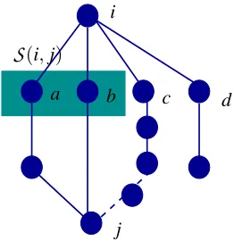
holds asymptotically almost surely4 (a.a.s.) with respect to the random-graph ensemble G(p). Our conditions and theoretical guarantees will be based on this notion for random graph ensembles. Intuitively, this means that graphs that have a vanishing prob-ability of occurrence asp→∞are ignored.We now characterize the ensemble of graphs amenable for consistent structure estimation under our formulation. To this end, we define the concept of local separation in graphs. See Fig. 1 for an illustration. Forγ∈N, letBγ(i;G)denote the set of vertices within distanceγfromiwith respect
to graphG. LetHγ,i:=G(Bγ(i))denote the subgraph ofGspanned byBγ(i;G), but in addition, we
retain the nodes not inBγ(i)(and remove the corresponding edges). Thus, the number of vertices in
Hγ,iisp.
Definition 1 (γ-Local Separator) Given a graph G, a γ-local separatorSγ(i,j) between i and j,
for (i,j)∈/ G, is aminimalvertex separator5 with respect to the subgraph Hγ,i. In addition, the
parameterγis referred to as thepath thresholdfor local separation.
In other words, theγ-local separatorSγ(i,j)separates nodesiand jwith respect to paths inGof
length at mostγ. We now characterize the ensemble of graphs based on the size of local separators.
Definition 2 ((η,γ)-Local Separation Property) An ensemble of graphs satisfies(η,γ)-local sep-aration property if for a.e. Gpin the ensemble,
max
(i,j)∈/Gp|
Sγ(i,j)| ≤η. (4)
We denote such a graph ensemble byG(p;η,γ).
In Section 3, we propose an efficient algorithm for graphical model selection when the under-lying graph belongs to a graph ensembleG(p;η,γ)with sparse local separators (i.e., smallη, forη
defined in (4)). We will see that the computational complexity of our proposed algorithm scales as O(pη+2). We now provide examples of several graph families satisfying (4).
4. Note that the term a.a.s. does not apply to deterministic graph ensemblesG(p)where no randomness is assumed, and in this setting, we assume that the propertyQ holds for every graph in the ensemble.
j
a b c d
i
S
(i,j)Figure 1: Illustration ofl-local separator set
S
(i,j;G,l)for the graph shown above withl=4. Note thatN
(i) ={a,b,c,d}is the neighborhood ofiand thel-local separator setS
(i,j;G,l) ={a,b} ⊂
N
(i;G). This is because the path alongcconnectingiand jhas a length greater thanland hence nodec∈/S
(i,j;G,l).2.2.1 EXAMPLE1: BOUNDED-DEGREE
We now show that the local-separation property holds for a rich class of graphs. Any (deterministic or random) ensemble of degree-bounded graphsGDeg(p,∆)satisfies(η,γ)-local separation property withη=∆and arbitraryγ∈N. If we do not impose any further constraints onGDeg, the computa-tional complexity of our proposed algorithm scales asO(p∆+2)(see also Bresler et al., 2008 where the computational complexity is comparable). Thus, when∆is large, our proposed algorithm and the one in Bresler et al. (2008) are computationally intensive. Our goal in this paper is to relax the usual bounded-degree assumption and to consider ensembles of graphsG(p)whose maximum degrees may grow with the number of nodesp. To this end, we discuss other structural constraints which can lead to graphs with sparse local separators.
2.2.2 EXAMPLE2: BOUNDEDLOCALPATHS
Another sufficient condition6 for the(η,γ)-local separation property in Definition 2 to hold is that there are at mostηpaths of length at mostγinGbetween any two nodes (henceforth, termed as the
(η,γ)-local paths property). In other words, there are at mostη−1 number of overlapping7cycles of length smaller than 2γ.
In particular, a special case of the local-paths property described above is the so-called girth property. Thegirthof a graph is the length of the shortest cycle. Thus, a graph with girthgsatisfies
(η,γ)-local separation property with η=1 and γ=g/2. LetGGirth(p;g)denote the ensemble of graphs with girth at most g. There are many graph constructions which lead to large girth. For example, the bipartite Ramanujan graph (Chung, 1997, p. 107) and the random Cayley graphs (Gamburd et al., 2009) have large girths.
6. For any graph satisfying(η,γ)-local separation property, the number of vertex-disjoint paths of length at mostγ
between any two non-neighbors is bounded above byη, by appealing to Menger’s theorem for bounded path lengths (Lov´asz et al., 1978). However, the property of local paths that we describe above is a stronger notion than having sparse local separators and we consider all distinct paths of length at mostγand not just vertex disjoint paths in the formulation.
The girth condition can be weakened to allow for a small number of short cycles, while not allowing for typical node neighborhoods to contain short cycles. Such graphs are termed aslocally tree-like. For instance, the ensemble of Erd˝os-R´enyi graphsGER(p,c/p), where an edge between any node pair appears with a probabilityc/p, independent of other node pairs, is locally tree-like. The parameterc may grow with p, albeit at a controlled rate for tractable structure learning. We make this more precise in Example 3 in Section 3.1. The proof of the following result may be found in Anandkumar et al. (2012a).
Proposition 3 (Random Graphs are Locally Tree-Like) The ensemble of Erd˝os-R´enyi graphs GER(p,c/p)satisfies the(η,γ)-local separation property in(4)with
η=2,γ≤ logp
4 logc. (5)
Thus, there are at most two paths of length smaller thanγbetween any two nodes in Erd˝os-R´enyi graphs a.a.s, or equivalently, there are no overlapping cycles of length smaller than 2γa.a.s. Simi-lar observations apply for the more generalscale-freeorpower-lawgraphs (Chung and Lu, 2006; Dommers et al., 2010). Along similar lines, the ensemble of ∆-random regular graphs, denoted byGReg(p,∆), which is the uniform ensemble of regular graphs with degree∆has no overlapping cycles of length at mostΘ(log∆−1p)a.a.s. (McKay et al., 2004, Lemma 1).
2.2.3 EXAMPLE3: SMALL-WORLDGRAPHS
The previous two examples showed local separation holds under two different conditions: bounded maximum degree and bounded number of local paths. The former class of graphs can have short cycles but the maximum degree needs to be constant, while the latter class of graphs can have a large maximum degree but the number of overlapping short cycles needs to be small. We now provide instances which incorporate both these features: large degrees and short cycles, and yet satisfy the local separation property.
The class of hybrid graphs or augmented graphs (Chung and Lu, 2006, Ch. 12) consists of graphs which are the union of two graphs: a “local” graph having short cycles and a “global” graph having small average distances. Since the hybrid graph is the union of these local and global graphs, it has both large degrees and short cycles. The simplest modelGWatts(p,d,c/p), first studied by Watts and Strogatz (1998), consists of the union of a d-dimensional grid and an Erd˝os-R´enyi random graph with parameter c. It is easily seen that a.e. graph G∼GWatts(p,d,c/p) satisfies
(η,γ)-local separation property in (4), with
η=d+2,γ≤ logp
4 logc.
Similar observations apply for more general hybrid graphs studied in Chung and Lu (2006, Ch. 12). Thus, we see that a wide range of graphs satisfy the property of having sparse local separators, and that it is possible for graphs with large degrees as well as many short cycles to have this property.
2.2.4 COUNTER-EXAMPLE: DENSEGRAPHS
number of edges scales super-linearly in the number of nodes. For instance, the Erd˝os-R´enyi graphs
GER(p,c/p) in the dense regime, where the average degree scales asc=Ω(p2). In this regime, the node degrees as well as the number of short cycles grow with p. However, there is no simple decomposition into a local and a global graph with desirable properties, as in the previous example of small world graphs. Thus, the size of the local separators also grows with pin this case. Such graphs are hard instances for our framework.
3. Guarantees for Conditional Covariance Thresholding
We now characterize conditions under which the underlying Markov structure can be recovered successfully under conditional covariance thresholding.
3.1 Assumptions
(A1) Sample Scaling Requirements: We consider the asymptotic setting where both the number of variables (nodes) p and the number of samples n tend to infinity. We assume that the parameters(n,p,Jmin)scale in the following fashion:8
n=Ω(Jmin−2logp). (6)
We require that the number of nodes p→∞to exploit the local separation properties of the class of graphs under consideration.
(A2) α-Walk-summability:The Gaussian graphical model Markov onGp∼G(p)isα-walk summable
a.a.s., that is,
kRGpk ≤α<1, a.e.Gp∼G(p), (7) whereαis a constant (i.e., not a function ofp),R:= [|R(i,j)|]is the entry-wise absolute value of the partial correlation matrixRandk·kdenotes the spectral norm.
(A3) Local-Separation Property: We assume that the ensemble of graphsG(p;η,γ)satisfies the
(η,γ)-local separation property withη,γsatisfying:
η=O(1), JminDmin−1α−γ=ω(1), (8) whereαis given by (7) andDmin:=miniJ(i,i)is the minimum diagonal entry of the potential
matrixJ.
(A4) Condition on Edge-Potentials:The minimum absolute edge potential of anα-walk summable Gaussian graphical model satisfies
Dmin(1−α) min
(i,j)∈Gp J(i,j)
K(i,j) >1+δ, (9)
for almost everyGp∼G(p), for someδ>0 (not depending on p) and9
K(i,j):=kJ(V\ {i,j},{i,j})k2, 8. The notationsω(·),Ω(·)refer to asymptotics as the number of variablesp→∞.
9. Here and in the sequel, forA,B⊂V, we use the notationJ(A,B)to denote the sub-matrix ofJindexed by rows inA
is the spectral norm of the submatrix of the potential matrixJ, andDmin:=miniJ(i,i)is the
minimum diagonal entry of J. Intuitively, (9) limits the extent of non-homogeneity in the model and the extent of overlap of neighborhoods. Moreover, this assumption is not required for consistent graphical model selection when the model is attractive (Ji,j≤0 fori6=j).10
(A5) Choice of thresholdξn,p: The thresholdξn,pfor graph estimation underCMITalgorithm is
chosen as a function of the number of nodes p, the number of samplesn, and the minimum edge potentialJminas follows:
ξn,p=O(Jmin),ξn,p=ω
αγ
Dmin
,ξn,p=Ω r
logp n
!
, (10)
whereαis given by (7), Dmin:=miniJ(i,i)is the minimum diagonal entry of the potential
matrixJ, andγis the path-threshold (4) for the(η,γ)-local separation property to hold.
Assumption (A1) stipulates how n, pandJminshould scale for consistent graphical model se-lection, that is, the sample complexity. The sample sizenneeds to be sufficiently large with respect to the number of variables p in the model for consistent structure reconstruction. Assumptions (A2) and (A4) impose constraints on the model parameters. Assumption (A3) restricts the class of graphs under consideration. To the best of our knowledge, all previous works dealing with graphi-cal model selection, for example, Meinshausen and B¨uhlmann (2006), Ravikumar et al. (2011), also impose some conditions for consistent graphical model selection. Assumption (A5) is with regard to the choice of a suitable thresholdξn,pfor thresholding conditional covariances. In the sequel, we
compare the conditions for consistent recovery after presenting our main theorem.
3.1.1 EXAMPLE1: DEGREE-BOUNDEDENSEMBLES
To gain a better understanding of conditions (A1)–(A5), consider the ensemble of graphsGDeg(p;∆)
with bounded degree∆∈N. It can be established that for the walk-summability condition in (A2)
to hold,11we require that for normalized precision matrices(J(i,i) =1), Jmax=O
1
∆
.
See Section A.2 for detailed discussion. When the minimum potential achieves the bound(Jmin=
Θ(1/∆)), a sufficient condition for (A3) to hold is given by
∆αγ=o(1), (11)
where γis the path threshold for the local-separation property to hold according to Definition 2. Intuitively, we require a larger path threshold γ, as the degree bound ∆ on the graph ensemble increases.
Note that (11) allows for the degree bound ∆ to grow with the number of nodes as long as the path threshold γ also grows appropriately. For example, if the maximum degree scales as
∆=O(poly(logp))and the path-threshold scales as γ=O(log logp), then (11) is satisfied. This implies that graphs with fairly large degrees and short cycles can be recovered successfully using our algorithm.
10. The assumption (A5) rules out the possibility that the neighbors are marginally independent. See Section B.3 for details.
3.1.2 EXAMPLE2: GIRTH-BOUNDEDENSEMBLES
The condition in (11) can be specialized for the ensemble of girth-bounded graphsGGirth(p;g)in a straightforward manner as
∆αg2 =o(1), (12)
wheregcorresponds to thegirthof the graphs in the ensemble. The condition in (12) demonstrates a natural tradeoff between the girth and the maximum degree; graphs with large degrees can be learned efficiently if their girths are large. Indeed, in the extreme case of trees which have infinite girth, in accordance with (12), there is no constraint on node degrees for successful recovery and recall that the Chow-Liu algorithm (Chow and Liu, 1968) is an efficient method for model selection on tree distributions.
3.1.3 EXAMPLE3: ERDOS˝ -R ´ENYI ANDSMALL-WORLDENSEMBLES
We can also conclude that a.e. Erd˝os-R´enyi graph G ∼ GER(p,c/p) satisfies (8) when c=O(poly(logp)) under the best-possible scaling ofJmin subject to the walk-summability con-straint in (7) (i.e.,Jminachieves the upper bound).
This is because it can be shown thatJmin=O(1/ √
∆)for walk-summability in (7) to hold. See Section A.2 for details. Noting that a.a.s., the maximum degree∆forG∼GER(p,c/p)satisfies
∆=O
logplogc log logp
,
from Bollob´as (1985, Ex. 3.6) and γ=O(loglogpc) from (5). Thus, the Erd˝os-R´enyi graphs are amenable to successful recovery when the average degree c=O(poly(logp)). Similarly, for the small-world ensemble GWatts(p,d,c/p), when d =O(1) and c=O(poly(logp)), the graphs are amenable for consistent estimation.
3.2 Consistency of Conditional Covariance Thresholding
Assuming (A1)–(A5), we now state our main result. The proof of this result and the auxiliary lemmata for the proof can be found in Sections B and Section C.
Theorem 4 (Structural consistency ofCMIT) For structure learning of Gaussian graphical
mod-els Markov on a graph Gp∼G(p;η,γ),CMIT(xn;ξn,p,η)is consistent for a.e. graph Gp. In other
words,
lim
n,p→∞
n=Ω(Jmin−2logp)
P[CMIT({xn};ξn,p,η)6=Gp] =0
Remarks:
2. Analysis of sample complexity: The above result states that the sample complexity for the CMIT(n=Ω(J−2
minlogp)), which improves when the minimum edge potentialJminis large.12 This is intuitive since the edges have stronger potentials in this case. On the other hand, Jmincannot be arbitrarily large since theα-walk-summability assumption in (7) imposes an upper bound onJmin. The minimum sample complexity (over different parameter settings) is attained whenJminachieves this upper bound. See Section A.2 for details. For example, for any degree-bounded graph ensembleG(p,∆)with maximum degree∆, the minimum sample complexity isn=Ω(∆2logp), that is, whenJ
min=Θ(1/∆), while for Erd˝os-R´enyi random graphs, the minimum sample complexity can be improved ton=Ω(∆logp), that is, when Jmin=Θ(1/
√
∆).
3. Comparison with Ravikumar et al. (2011): The work by Ravikumar et al. (2011) employs an
ℓ1-penalized likelihood estimator for structure estimation in Gaussian graphical models. Un-der the so-called incoherence conditions, the sample complexity isn=Ω((∆2+J−2
min)logp). Our sample complexity in (6) is the same in terms of its dependence onJmin, and there is no explicit dependence on the maximum degree∆. Moreover, we have a transparent sufficient condition in terms ofα-walk-summability in (7), which directly imposes scaling conditions on Jmin. It is an open question if the models satisfying incoherence conditions are walk-summable or viceversa. However, for random graph models, we can obtain better guarantees in terms of average degrees while the incoherence conditions are based on maximum degree in the graph. We also present experimental comparison between this method and our developed method in Section 6.
4. Comparison with Meinshausen and B¨uhlmann (2006): The work by
Meinshausen and B¨uhlmann (2006) considers ℓ1-penalized linear regression for neighbor-hood selection of Gaussian graphical models and establish a sample complexity ofn=Ω((∆+ Jmin−2)logp). We note that our guarantees allow for graphs which do not necessarily satisfy the conditions imposed by Meinshausen and B¨uhlmann (2006). For instance, the assumption of neighborhood stability (assumption 6 in Meinshausen and B¨uhlmann, 2006) is hard to ver-ify in general, and the relaxation of this assumption corresponds to the class of models with diagonally-dominant covariance matrices. Note that the class of Gaussian graphical mod-els with diagonally-dominant covariance matrices forms a strict sub-class of walk-summable models, and thus satisfies assumption (A2) for the theorem to hold. Thus, Theorem 4 ap-plies to a larger class of Gaussian graphical models compared to Meinshausen and B¨uhlmann (2006). Furthermore, the conditions for successful recovery in Theorem 4 are arguably more transparent.
5. Local vs. Global Conditions for Success: The conditions required for the success of our methods as well as the ℓ1 penalized MLE of Ravikumar et al. (2011) are global, meaning that the entire model (i.e., all the parameters) need to satisfy the specified conditions for recovering the entire graph. It does not appear straightforward to characterize local conditions for successful recovery under our formulation, that is, when our algorithm may succeed in recovering some parts of the graph, but not others. On the other hand, the ℓ1 penalized neighborhood selection method of Meinshausen and B¨uhlmann (2006) provides a separate
set of conditions for recovery of each neighborhood in the graph. However, as discussed above, these conditions appear stronger and more opaque than our conditions.
6. Comparison with Ising models: Our above result for learning Gaussian graphical models is analogous to structure estimation of Ising models subject to an upper bound on the edge potentials (Anandkumar et al., 2012b), and we characterize such a regime as aconditional uniquenessregime. Thus, walk-summability is the analogous condition for Gaussian models.
Proof Outline:We first analyze the scenario when exact statistics are available. (i) We establish that for any two non-neighbors(i,j)∈/ G, the minimum conditional covariance in (1) (based on exact statistics) does not exceed the thresholdξn,p. (ii) Similarly, we also establish that the conditional
covariance in (1) exceeds the thresholdξn,pfor all neighbors(i,j)∈G. (iii) We then extend these
results to empirical versions using concentration bounds.
3.2.1 PERFORMANCE OFCONDITIONALMUTUALINFORMATIONTEST
We now employ the conditional mutual information test, analyzed in Anandkumar et al. (2012b) for Ising models, and note that it has slightly worse sample complexity than using conditional co-variances. Using the thresholdξn,pdefined in (10), the conditional mutual information testCMITis
given by the threshold test
min
S⊂V\{i,j} |S|≤η
b
I(Xi;Xj|XS)>ξ2n,p,
and node pairs(i,j)exceeding the threshold are added to the estimateGbnp. Assuming (A1)–(A5), we have the following result.
Theorem 5 (Structural consistency ofCMIT) For structure learning of the Gaussian graphical
model on a graph Gp ∼G(p;η,γ), CMIT(xn;ξn,p,η) is consistent for a.e. graph Gp. In other
words,
lim
n,p→∞
n=Ω(Jmin−4logp)
P[CMIT({xn};ξn,p,η)6=Gp] =0
The proof of this theorem is provided in Section C.3. Remarks:
1. For Gaussian random variables, conditional covariances and conditional mutual information are equivalent tests for conditional independence. However, from above results, we note that there is a difference in the sample complexity for the two tests. The sample complexity of CMIT isn=Ω(J−4
minlogp) in contrast ton=Ω(J− 2
minlogp) forCMIT. This is due to faster decay of conditional mutual information on the edges compared to the decay of conditional covariances. Thus, conditional covariances are more efficient for Gaussian graphical model selection compared to conditional mutual information.
4. Necessary Conditions for Model Selection
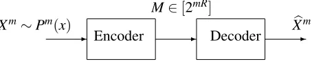
- - -Xm∼Pm(x)
Encoder
M∈[2mR]
Decoder Xb
m
Figure 2: The canonical source coding problem. See Chapter 3 in Cover and Thomas (2006).
For the class of degree-bounded graphsGDeg(p,∆), necessary conditions on sample complexity have been characterized before (Wang et al., 2010) by considering a certain (limited) set of ensem-bles. However, a na¨ıve application of such bounds (based on Fano’s inequality (Cover and Thomas, 2006, Ch. 2)) turns out to be too weak for the class of Erd˝os-R´enyi graphsGER(p,c/p), where the average degree13cis much smaller than the maximum degree.
We now provide necessary conditions on the sample complexity for recovery of Erd˝os-R´enyi graphs. Our information-theoretic techniques may also be applicable to other ensembles of random graphs. This is a promising avenue for future work.
4.1 Setup
We now describe the problem more formally. A graphGis drawn from the ensemble of Erd˝os-R´enyi graphsG∼GER(p,c/p). The learner is also provided withn conditionally i.i.d. samples Xn := (X1, . . . ,Xn)∈(
X
p)n (whereX
=R) drawn from the conditional (Gaussian) product probabilitydensity function (pdf)∏ni=1f(xi|G). The task is then to estimateG, a random quantity. The estimate
is denoted asGb:=Gb(Xn). It is desired to derive tight necessary conditions onn(as a function ofc andp) so that theprobability of error
Pe(p):=P(Gb6=G)→0 (13)
as the number of nodesptends to infinity. Note that the probability measurePin (13) is associated toboththe realization of the random graphGand the samplesXn.
The task is reminiscent of source coding (or compression), a problem of central importance in information theory (Cover and Thomas, 2006)—we would like to derive fundamental limits associ-ated to the problem of reconstructing the sourceGgiven a compressed version of itXn(Xnis also analogous to the “message”). However, note the important distinction; while in source coding, the source coder can design both the encoderandthe decoder, our problem mandates that the code is fixed by the conditional probability density f(x|G). We are only allowed to design the decoder. See comparisons in Figs. 2 and 3.
4.2 Necessary Conditions for Exact Recovery
To derive the necessary condition for learning Gaussian graphical models Markov on sparse Erd˝os-R´enyi graphsG∼GER(p,c/p), we assume that the strict walk-summability condition with param-eterα, according to (7). We are then able to demonstrate the following:
Theorem 6 (Weak Converse for Gaussian Models) For a walk-summable Gaussian graphical model satisfying(7)with parameterα, for almost every graph G∼GER(p,c/p)as p→∞, in order
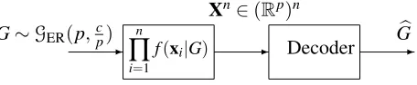
- - -G∼GER(p,cp) n
∏
i=1
f(xi|G)
Xn∈(Rp)n
Decoder Gb
Figure 3: The estimation problem is analogous to source coding: the “source” isG∼GER(p,c p),
the “message” is Xn∈(Rp)n and the “decoded source” is Gb. We are asking what the
minimum “rate” (analogous to the number of samplesn) are required so thatGb=Gwith high probability.
for Pe(p)→0, we require that
n≥ 2
plog22πe 1−1α+1
p 2
Hb
c p
(14)
for all p sufficiently large.
The proof is provided in Section D.1. By expanding the binary entropy function, it is easy to see that the statement in (14) can be weakened to the necessary condition:
n≥ clog2p
log22πe 1−1α+1.
The above condition does not involve any asymptotic notation, and also demonstrates the depen-dence of the sample complexity on p,candαtransparently. Finally, the dependence onαcan be explained as follows: anyα-walk-summable model is alsoβ-walk-summable for allβ>α. Thus, the class ofβ-walk-summable models contains the class ofα-walk-summable models. This results in a looser bound in (14) for largerα.
4.3 Necessary Conditions for Recovery with Distortion
In this section, we generalize Theorem 6 to the case where we only require estimation of the under-lying graph up to a certain edit distance: an error is declared if and only if the estimated graphGb exceeds an edit distance (or distortion)Dof the true graph. Theedit distance d:Gp×Gp→N∪{0}
between two undirected graphsG= (V,E)andG= (V,E′)is defined asd(G,G′):=|E△E′|, where △ denotes the symmetric difference between the edge setsE andE′. The edit distance can be regarded as a distortion measure between two graphs.
Given an positive integerD, known as thedistortion, suppose we declare an error if and only if d(G,G′)>D, then the probability of error is redefined as
Pe(p):=P(d(G,Gb(Xn))>D). (15)
We derive necessary conditions onn(as a function ofpandc) such that the probability of error (15) goes to zero asp→∞. To ease notation, we define the ratio
β:=D/
p 2
. (16)
Corollary 7 (Weak Converse for Discrete Models With Distortion) For Pe(p)→0, we must have
n≥ 2
plog22πe 1−1α+1
p 2 Hb c p
−Hb(β)
(17)
for all p sufficiently large.
The proof of this corollary is provided in Section D.7. Note that for (17) to be a useful bound, we needβ<c/pwhich translates to an allowed distortionD<cp/2. We observe from (17) that because the error criterion has been relaxed, the required number of samples is also reduced from the corresponding lower bound in (14).
4.4 Proof Techniques
Our analysis tools for deriving necessary conditions for Gaussian graphical model selection are information-theoretic in nature. A common and natural tool to derive necessary conditions (also called converses) is to resort to Fano’s inequality (Cover and Thomas, 2006, Chapter 2), which (lower) bounds the probability of errorPe(p)as a function of theequivocationorconditional entropy
H(G|Xn)and the size of the set of all graphs withpnodes. However, a direct and na¨ıve application Fano’s inequality results in a trivial lower bound as the set of all graphs, which can be realized by
GER(p,c/p)is, loosely speaking, “too large”.
To ameliorate such a problem, we employ another information-theoretic notion, known as typi-cality. Atypical setis, roughly speaking, a set that has small cardinality and yet has high probability asp→∞. For example, the probability of a set of length-msequences is of the order≈2mH (where H is the entropy rate of the source) and hence those sequences with probability close to this value are calledtypical. In our context, given a graphG, we define the ¯d(G)to be the ratio of the number of edges ofGto the total number of nodes p. LetGpdenote the set of all graphs with pnodes. For
a fixedε>0, we define the following set of graphs:
T
ε(p):=
G∈Gp:
¯ d(G)
c − 1 2 ≤ ε 2 .
The set
T
ε(p)is known as theε-typical set of graphs. Every graphG∈T
ε(p)has an average number of edges that is c2ε-close in the Erd˝os-R´enyi ensemble. Note that typicality ideas are usually used to derive sufficientconditions in information theory (Cover and Thomas, 2006) (achievability in information-theoretic parlance); our use ofbothtypicality for graphical model selection as well as Fano’s inequality to derive converse statements seems novel. Indeed, the proof of the converse of the source coding theorem in Cover and Thomas (2006, Chapter 3) uses only Fano’s inequality. We now summarize the properties of the typical set.Lemma 8 (Properties of
T
ε(p)) Theε-typical set of graphs has the following properties:1. P(
T
ε(p))→1as p→∞.2. For all G∈
T
ε(p), we have14exp2 − p 2 Hb c p (1+ε)
≤P(G)≤exp2
− p 2 Hb c p .
3. The cardinality of theε-typical set can be bounded as
(1−ε)exp2
p 2
Hb
c p
≤ |
T
ε(p)| ≤exp2
p 2
Hb
c p
(1+ε)
for all p sufficiently large.
The proof of this lemma can be found in Section D.2. Parts 1 and 3 of Lemma 8 respectively say that the set of typical graphs has high probability and has very small cardinality relative to the number of graphs withpnodes|Gp|=exp2( p
2
). Part 2 of Lemma 8 is known as theasymptotic equipartition property: the graphs in the typical set are almost uniformly distributed.
5. Implications on Loopy Belief Propagation
An active area of research in the graphical model community is that of inference—that is, the task of computing node marginals (or MAP estimates) through efficient distributed algorithms. The simplest of these algorithms is the belief propagation15(BP) algorithm, where messages are passed among the neighbors of the graph of the model. It is known that belief propagation (and max-product) is exact on tree models, meaning that correct marginals are computed at all the nodes (Pearl, 1988). On the other hand on general graphs, the generalized version of BP, known as loopy belief propagation (LBP), may not converge and even if it does, the marginals may not be correct. Motivated by the twin problems of convergence and correctness, there has been extensive work on characterizing LBP’s performance for different models. As a by-product of our previous analysis on graphical model selection, we now show the asymptotic correctness of LBP on walk-summable Gaussian models when the underlying graph is locally tree-like.
5.1 Background
The belief propagation (BP) algorithm is a distributed algorithm where messages (or beliefs) are passed among the neighbors to draw inferences at the nodes of a graphical model. The computa-tion of node marginals through na¨ıve variable eliminacomputa-tion (or Gaussian eliminacomputa-tion in the Gaussian setting) is prohibitively expensive. However, if the graph is sparse (consists of few edges), the com-putation of node marginals may be sped up dramatically by exploiting the graph structure and using distributed algorithms to parallelize the computations.
For the sake of completeness, we now recall the basic steps in LBP, specific to Gaussian graph-ical models. Given a message schedule which specifies how messages are exchanged, each node j receives information from each of its neighbors (according to the graph), where the message, mti→j(xj), fromito j, intthiteration is parameterized as
mti→j(xj):=exp
−12∆Jit→jx2j+∆hti→jxj
.
Each node i prepares message mti→j(xj) by collecting messages from neighbors of the previous
iteration (under parallel iterations), and computing
ˆ
Ji\j(t) =J(i,i) +
∑
k∈N(i)\j∆Jkt−→1i, hˆi\j(t) =h(i) +
∑
k∈N(i)\j∆hk→i(t),
where
∆Jit→j=−J(j,i)Jˆ−1
i\j(t)J(j,i), ∆h t
i→j=−J(j,i)Jˆi−\1j(t)hˆk→i(t). 5.2 Results
LetΣLBP(i,i)denote the variance at nodeiat the LBP fixed point.16 Without loss of generality, we consider the normalized version of the precision matrix
J=I−R,
which can always be obtained from a general precision matrix via normalization. We can then renor-malize the variances, computed via LBP, to obtain the variances corresponding to the unnorrenor-malized precision matrix.
We consider the following ensemble of locally-tree like graphs. Consider the event that the neighborhood of a nodeihas no cycles up to graph distanceγ, given by
Γ(i;γ,G):={Bγ(i;G)does not contain any cycles}.
We assume a random graph ensembleG(p)such that for a given nodei∈V, we have
P[Γc(i;γ,G)] =o(1). (18)
Proposition 9 (Correctness of LBP) Given an α-walk-summable Gaussian graphical model on a.e. locally tree-like graph G∼G(p;γ)with parameterγsatisfying(18), we have
|ΣG(i,i)−ΣLBP(i,i)|a.a.s.= O(max(αγ,P[Γc(i;γ,G)])). The proof is given in Section B.4.
Remarks:
1. The class of Erd˝os-R´enyi random graphs, G ∼ GER(p,c/p) satisfies (18), with
γ=O(logp/logc)for a nodei∈V chosen uniformly at random.
2. Recall that the class of random regular graphsG∼GReg(p,∆) have a girth ofO(log∆−1p). Thus, for any nodei∈V, (18) holds withγ=O(log∆−1p).
6. Experiments
In this section we present some experimental results on real and synthetic data. We implement the proposedCMITmethod as well the convex relaxation methods, namely, theℓ1penalized maxi-mum likelihood estimate (MLE) (Ravikumar et al., 2011) andℓ1penalized neighborhood selection (Meinshausen and B¨uhlmann, 2006). We measure the performance of methods using the notion of the edit distance between the true and estimated graphs (for synthetic data). We also compare the penalized likelihood scores of the estimated models using the notion of Bayesian information criterion (BIC) for both synthetic and real data. We implement the proposed CMIT method in MATLAB and the convex relaxation methods using the YALMIP package.17 We also used CON-TEST18 to generate the synthetic graphs. The data sets, software code and results are available at
http://newport.eecs.uci.edu/anandkumar.
6.1 Data Sets
Synthetic data:In order to evaluate the performance of our algorithm in terms of error in reconstruct-ing the graph structure, we generated samples from Gaussian graphical models for different graphs. These include a single cycle graph withp=80 nodes, an Erd˝os-R´enyi (ER) graphG∼GER(p,c/p) with average degreec=1.2 and Watts-Strogatz modelGWatts(p,d,c/p)with degree of local graph d=2 and average degree of the global graph c=1.2. Given the graph structureG, we generate the potential matrix JG whose sparsity pattern corresponds to that ofG. We set the diagonal
el-ements inJG to unity and nonzero off-diagonal entries are picked uniformly19 from [0,0.1]. We
set the potential vector h to be 0 without loss of generality. We let the number of samples be n∈ {102,5×102,103,5×103,104}. Note that for synthetic data, we knowη, the size of local sep-arators for non-neighboring node pairs in the graph, and we incorporate it in the implementation of theCMIT algorithm. We present edit distance results forCMITand the above mentioned convex relaxation methods for different thresholds and regularization parameters.20
Foreign exchange data: We consider monthly trends of foreign exchange rates21of 19 curren-cies22 with respect to the US dollar from 10/1/1983 to 02/1/2012. We evaluate the BIC score for models estimated using our algorithm under different thresholdsξn,pand different sizes of the local
separator setsη, and compared it with the convex relaxation methods under different regularization parameters.
6.2 Performance Criteria
The BIC score has been extensively used to enable tradeoff between data fitting and model com-plexity (Schwarz, 1978). We use a modified version of the BIC score proposed for high-dimensional data sets (Foygel and Drton, 2010) as the performance criterion for model fitting. Givennsamples
xn:= [x
1, . . . ,xn], and parametersθ,
BIC(xn;θ):= n
∑
k=1logf(xk;θ)−0.5|E|logn−2|E|logp,
where|E|is the number of edges in the Markov graph andθis the set of parameters characterizing
the model. It has been observed elsewhere (Liu et al., 2009) that the BIC score tends to overselect the edges leading to dense graphs, and thus, we impose a hard threshold on the number of edges (both for our method and for convex relaxation methods), and select the model with the best BIC score. For the foreign exchange data, we limited the number of edges to 100, while for synthetic data, we limited it to 100 for cycle and Erd˝os-R´enyi (ER) graphs and to 200 for the Watts-Strogatz model. We note that alternatively, the thresholds/regularization parameters can be selected via cross validation or other mechanisms, see Liu et al. (2009) for details.
19. The choice of parameters and graphs result in valid models in our experiments, that is, the potential matrix is positive definite.
20. For the convex relaxation methods in Ravikumar et al. (2011) and Meinshausen and B¨uhlmann (2006), the regular-ization parameter denotes the weight associated with theℓ1term.
Graph n CMIT ℓ1MLE ℓ1Nbd Cycle 102 1.0000 1.0000 1.0000 ER 102 1.0000 1.0000 1.0000 WS 102 1.0000 1.0000 1.0000 Cycle 103 0.95 0.9875 0.9000 ER 103 0.6825 1.1087 1.0000 WS 103 0.8580 0.9520 0.8063 Cycle 104 0.4125 0.3875 0.3625 ER 104 0.3273 0.3469 0.5435 WS 104 0.3252 0.3313 0.2688
Table 1: Normalized edit distance underCMIT,ℓ1penalized MLE andℓ1penalized neighborhood selection on synthetic data from graphs listed above, wherendenotes the number of sam-ples.
6.3 Experimental Outcomes
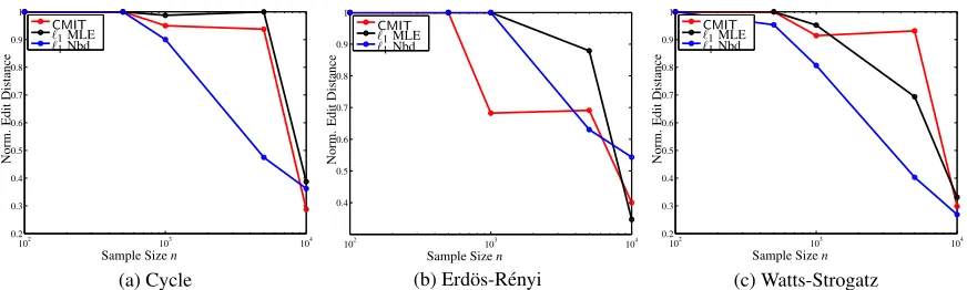
Synthetic data:We compare the performance of our methodCMITwith convex relaxation methods for synthetic data as described earlier. We evaluate the normalized edit distance (normalized with respect to the number of edges), since we know the ground truth for synthetic data and present the results in Table 1 forCMIT,ℓ1penalized MLE andℓ1penalized neighborhood selection. methods. The results are also presented in figures 7a, 7b and 7c. We note thatCMIThas better edit distance performance and BIC scores compared toℓ1penalized MLE in most cases, and similar performance compared to theℓ1penalized neighborhood selection.
Foreign exchange data: We evaluate the BIC scores under our algorithm CMIT with differ-ent values ofη (the constraint on the size of subsets used for conditioning)23 and thresholdξ
n,p.
We present the results in Table 2, where for each value ofη, we present the thresholdξn,p which
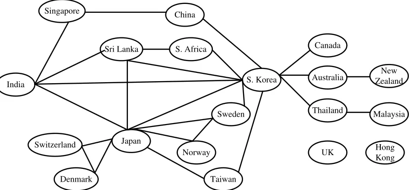
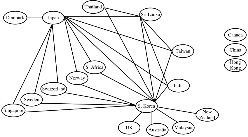
achieves the best BIC score under the sparsity constraint. We also present the regularization param-eters for convex relaxation methods with the best BIC. The estimated graphs are shown in figures 4 and 5. We note that whileCMIT distributes the edges fairly uniformly across the nodes, theℓ1 penalized MLE tends to cluster all the edges together between the “dominant” variables leading to a densely connected component and several isolated nodes. We observe from the reconstructed graphs that geography plays a crucial role in the foreign exchange trends. In Fig.4 recovered us-ing the CMIT method, we note that among Asian countries India and S. Korea are high degree nodes and are connected to countries which are geographically close (e.g., Sri Lanka for India, and Australia, Thailand, Taiwan and China for S. Korea). On the other hand, the ℓ1 method outputs a densely connected graph where such geographical relationships are missing. Thus, we see that in the experiments, the proposedCMITmethod tends to enforce local sparsity in the graph, while theℓ1 method of Ravikumar et al. (2011) enforces global sparsity, and tends to cluster the edges together. On the other hand, theℓ1penalized neighborhood selection (Meinshausen and B¨uhlmann, 2006) is better than the MLE in distributing the edges across all the nodes, but carries this out to a lesser extent than our method.
Thres.(CMIT) η LL-train×107 LL-test×107 BIC-train×107 BIC-test×107 |E|
0.5 1 -2.9521 -7.4441 -2.9522 -7.4442 23
0.5 2 -3.2541 -8.5923 -3.2541 -8.5923 8
0.01 3 -2.9669 -7.3773 -2.9670 -7.3774 19
0.001 4 -2.9653 -7.3674 -2.9654 -7.3675 25
0.0005 5 -3.2901 -8.8396 -3.3068 -8.8397 24
0.0005 6 -3.2921 -8.8466 -3.2921 -8.8467 18
Thres.(ℓ1MLE) − LL-train×107 LL-test×107 BIC-train×107 BIC-test×107 |E|
6.5803 − -2.5831 -6.3167 -2.5832 -6.3167 28
Thres.(ℓ1Nbd) − LL-train×107 LL-test×107 BIC-train×107 BIC-test×107 |E| 13.1606 − -2.7971 -6.9630 -2.7972 -6.9631 26
Table 2: Experimental outcome forCMIT,ℓ1penalized MLE andℓ1penalized neighborhood selec-tion for different thresholds/regularizaselec-tion parameters and size of condiselec-tioning setsηfor foreign exchange data.|E|denotes the number of edges.
India
Japan
S. Korea
Sri Lanka Canada China
Sweden S. Africa
Taiwan
Thailand
Australia ZealandNew
UK Hong Kong
Denmark
Malaysia
Norway Switzerland
Singapore
Figure 4: Graph estimate under CMITalgorithm for foreign exchange data set forη=4, see Ta-ble 2.
7. Conclusion
India Japan
S. Korea
Sri Lanka
Canada China
Sweden S. Africa
Taiwan Thailand
Australia
New Zealand
UK
Hong Kong
Denmark
Malaysia
Norway Switzerland
Singapore
Figure 5: Graph estimate underℓ1penalized MLE for foreign exchange data set. See Table 2.
India Japan
S. Korea Sri Lanka
Canada
China
Sweden
S. Africa
Taiwan Thailand
Australia
New Zealand
UK
Hong Kong Denmark
Malaysia Norway
Switzerland
Singapore
102 103 104 0.2 0.3 0.4 0.5 0.6 0.7 0.8 0.9 1 Sample Sizen N o rm . E d it D is ta n ce CMIT
ℓ1MLE
ℓ1Nbd
(a) Cycle
102 103 104
0.4 0.5 0.6 0.7 0.8 0.9 1 Sample Sizen N o rm . E d it D is ta n ce CMIT
ℓ1MLE
ℓ1Nbd
(b) Erd¨os-R´enyi 102 103 104 0.2 0.3 0.4 0.5 0.6 0.7 0.8 0.9 1
Sample Sizen
N o rm . E d it D is ta n ce CMIT
ℓ1MLE
ℓ1Nbd
(c) Watts-Strogatz
Figure 7:CMIT,ℓ1penalized MLE andℓ1penalized neighborhood selection methods.
Acknowledgments
An abridged version of this paper appeared in the Proceedings of NIPS 2011. The first author is supported in part by the setup funds at UCI and the AFOSR Award FA9550-10-1-0310, the second author is supported by A*STAR, Singapore and the third author is supported in part by AFOSR under Grant FA9550-08-1-1080. The authors thank Venkat Chandrasekaran (UC Berkeley) for discussions on walk-summable models, Elchanan Mossel (UC Berkeley) for discussions on the necessary conditions for model selection and Divyanshu Vats (U. Minn.) for extensive comments. The authors thank the Associate Editor Martin Wainwright (Berkeley) and the anonymous reviewers for comments which significantly improved this manuscript.
Appendix A. Walk-summable Gaussian Graphical Models
We first provide an overview of the notion of walk-summability for Gaussian graphical models.
A.1 Background on Walk-Summability
We now recap the properties of walk-summable Gaussian graphical models, as given by (7). For details, see Malioutov et al. (2006). For simplicity, we first assume that the diagonal of the potential matrixJis normalized (J(i,i) =1 for alli∈V). We remove this assumption and consider general unnormalized precision matrices in Section B.2. Consider splitting the matrixJ into the identity matrix and the partial correlation matrixR, defined in (3):
J=I−R. (19)
The covariance matrixΣof the graphical model in (19) can be decomposed as
Σ=J−1= (I−R)−1=
∞
∑
k=0Rk, kRk<1, (20)
using Neumann power series for the matrix inverse. Note that we require thatkRk<1 for (20) to hold, which is implied by walk-summability in (7) (sincekRk ≤ kRk).
denote the length of the walk. Given matrixRGsupported on graphG, let the weight of the walk be
φ(w):= |w|
∏
k=1R(wk−1,wk).
The elements of the matrix powerRl are given by
Rl(i,j) =
∑
w:i→l j
φ(w), (21)
wherei→l jdenotes the set of walks fromito jof lengthl. For this reason, we henceforth refer to
Ras thewalk matrix.
Leti→ jdenote all the walks betweeniand j. Under the walk-summability condition in (7), we have convergence of∑w:i→jφ(w), irrespective of the order in which the walks are collected, and
this is equal to the covarianceΣ(i,j).
In Section A.3, we relate walk-summability in (7) to the notion of correlation decay, where the effect of faraway nodes on covariances can be controlled and the local-separation property of the graphs under consideration can be exploited.
A.2 Sufficient Conditions for Walk-summability
We now provide sufficient conditions and suitable parameterization for walk-summability in (7) to hold. The adjacency matrixAGof a graphGwith maximum degree∆Gsatisfies
λmax(AG)≤∆G,
since it is dominated by a∆-regular graph which has maximum eigenvalue of ∆G. From
Perron-Frobenius theorem, for adjacency matrixAG, we haveλmax(AG) =kAGk, wherekAGkis the
spec-tral radius ofAG. Thus, forRGsupported on graphG, we have
α:=kRGk=O(Jmax∆), whereJmax:=maxi,j|R(i,j)|. This implies that
Jmax=O
1
∆
to haveα<1, which is the requirement for walk-summability.
When the graph G is a Erd˝os-R´enyi random graph, G∼GER(p,c/p), we can provide better bounds. WhenG∼GER(p,c/p), we have Krivelevich and Sudakov (2003), that
λmax(AG) = (1+o(1))max( p
∆G,c),
where∆Gis the maximum degree andAGis the adjacency matrix. Thus, in this case, whenc=O(1),
we require that
Jmax=O
r
1
∆ !
,
A.3 Implications of Walk-Summability
Recall thatΣG denotes the covariance matrix for Gaussian graphical model on graphGand that JG=Σ−G1 with JG=I−RG in (19). We now relate the walk-summability condition in (7) to
correlation decay in the model. In other words, under walk-summability, we can show that the effect of faraway nodes on covariances decays with distance, as made precise in Lemma 10.
LetBγ(i)denote the set of nodes withinγhops from nodeiin graphG. DenoteHγ;i j:=G(Bγ(i)∩
Bγ(j))as the induced subgraph ofG over the intersection ofγ-hop neighborhoods at iand jand
retaining the nodes inV\ {Bγ(i)∩Bγ(j)}. Thus,Hγ;i j has the same number of nodes asG. We first
make the following simple observation: the(i,j)element in theγthpower of walk matrix,Rγ
G(i,j), is
given by walks of lengthγbetweeniand jon graphGand thus, depends only on subgraph24Hγ;i j,
see (21). This enables us to quantify the effect of nodes outsideBγ(i)∩Bγ(j) on the covariance
ΣG(i,j).
Define a new walk matrixRHγ;i j such that
RHγ;i j(a,b) =
R
G(a,b), a,b∈Bγ(i)∩Bγ(j),
0, o.w.
In other words,RHγ;i j is formed by considering the Gaussian graphical model over graphHγ;i j. Let
ΣHγ;i j denote the corresponding covariance matrix. 25
Lemma 10 (Covariance Bounds Under Walk-summability) For any walk-summable Gaussian graphical model(α:=kRGk<1), we have26
max
i,j |ΣG(i,j)−ΣHγ;i j(i,j)| ≤α
γ 2α
1−α =O(α
γ). (22)
Thus, for walk-summable Gaussian graphical models, we have α:=kRGk<1, implying that
the error in (22) in approximating the covariance by local neighborhood decays exponentially with distance. Parts of the proof below are inspired by Dumitriu and Pal (2009).
Proof: Using the power-series in (20), we can write the covariance matrix as
ΣG=
γ
∑
k=0RkG+EG,
where the error matrixEGhas spectral radius
kEGk ≤ k RGkγ+1
1− kRGk ,
from (20). Thus,27for anyi,j∈V, |ΣG(i,j)−
γ
∑
k=0RkG(i,j)| ≤ kRGk
γ+1 1− kRGk
. (23)
24. Note thatRγ(i,j) =0 ifBγ(i)∩Bγ(j) =/0.
25. WhenBγ(i)∩Bγ(j) =/0meaning that graph distance betweeniand jis more thanγ, we obtainΣHγ;i j=I. 26. The bound in (22) also holds ifHγ;i jis replaced with any of its supergraphs.
Similarly, we have
|ΣHγ;i j(i,j)−
γ
∑
k=0RkHγ;i j(i,j)| ≤ kRHγ;i jk
γ+1 1− kRHγ;i jk
(a)
≤ kRGk
γ+1 1− kRGk
, (24)
where for inequality (a), we use the fact that
kRHγ;i jk ≤ kRHγ;i jk ≤ kRGk,
sinceHγ;i j is a subgraph28ofG.
Combining (23) and (24), using the triangle inequality, we obtain (22). 2 We also make some simple observations about conditional covariances in walk-summable mod-els. Recall thatRGdenotes matrix with absolute values ofRG, andRGis the walk matrix over graph
G. Also recall that theα-walk summability condition in (7), iskRGk ≤α<1.
Proposition 11 (Conditional Covariances under Walk-Summability) Given a walk-summable Gaussian graphical model, for any i,j∈V and S⊂V with i,j∈/S, we have
Σ(i,j|S) =
∑
w:i→j ∀k∈w,k∈/S
φG(w). (25)
Moreover, we have
sup
i∈V S⊂V\i
Σ(i,i|S)≤(1−α)−1=O(1). (26)
Proof: We have, from Rue and Held (2005, Thm. 2.5),
Σ(i,j|S) =J−−S1,−S;G(i,j),
where J−S,−S;G denotes the submatrix of potential matrixJG by deleting nodes inS. Since
sub-matrix of a walk-summable sub-matrix is walk-summable, we have (25) by appealing to the walk-sum expression for conditional covariances.
For (26), let kAk∞ denote the maximum absolute value of entries in matrix A. Using
mono-tonicity of spectral norm and the fact thatkAk∞≤ kAk, we have
sup
i∈V S⊂V,i∈/V
Σ(i,i|S)≤ kJ−−1S,−S;Gk= (1− kR−S,−S;Gk)−1
≤(1− kR−S,−S;Gk)−1≤(1− kRGk)−1=O(1).
2 Thus, the conditional covariance in (25) consists of walks in the original graphG, not passing through nodes inS.