Multi-task Regression using Minimal Penalties

(1)

Multi-task Regression using Minimal Penalties

Matthieu Solnon [email protected]

ENS; Sierra Project-team

Département d’Informatique de l’ École Normale Supérieure (CNRS/ENS/INRIA UMR 8548)

23, avenue d’Italie, CS 81321 75214 Paris Cedex 13, France

Sylvain Arlot [email protected]

CNRS; Sierra Project-team

Francis Bach [email protected]

INRIA; Sierra Project-team

Editor: Tong Zhang

Abstract

In this paper we study the kernel multiple ridge regression framework, which we refer to as multi-task regression, using penalization techniques. The theoretical analysis of this problem shows that the key element appearing for an optimal calibration is the covariance matrix of the noise between the different tasks. We present a new algorithm to estimate this covariance matrix, based on the concept of minimal penalty, which was previously used in the single-task regression framework to estimate the variance of the noise. We show, in a non-asymptotic setting and under mild as-sumptions on the target function, that this estimator converges towards the covariance matrix. Then plugging this estimator into the corresponding ideal penalty leads to an oracle inequality. We illus-trate the behavior of our algorithm on synthetic examples.

Keywords: multi-task, oracle inequality, learning theory

1. Introduction

(2)

One-dimensional kernel ridge regression, which we refer to as “single-task” regression, has been widely studied. As we briefly review in Section 3 one has, given n data points(Xi,Yi)n_i₌₁, to estimate

a function f , often the conditional expectation f(Xi) =E[Yi|Xi], by minimizing the quadratic risk

of the estimator regularized by a certain norm. A practically important task is to calibrate a regu-larization parameter, that is, to estimate the reguregu-larization parameter directly from data. For kernel ridge regression (a.k.a. smoothing splines), many methods have been proposed based on different principles, for example, Bayesian criteria through a Gaussian process interpretation (see, e.g., Ras-mussen and Williams, 2006) or generalized cross-validation (see, e.g., Wahba, 1990). In this paper, we focus on the concept of minimal penalty, which was first introduced by Birg´e and Massart (2007) and Arlot and Massart (2009) for model selection, then extended to linear estimators such as kernel ridge regression by Arlot and Bach (2011).

In this article we consider p_≥2 different (but related) regression tasks, a framework we refer to as “multi-task” regression. This setting has already been studied in different papers. Some em-pirically show that it can lead to performance improvement (Thrun and O’Sullivan, 1996; Caruana, 1997; Bakker and Heskes, 2003). Liang et al. (2010) also obtained a theoretical criterion (unfortu-nately non observable) which tells when this phenomenon asymptotically occurs. Several different paths have been followed to deal with this setting. Some consider a setting where p_≫n, and

formu-late a sparsity assumption which enables to use the group Lasso, assuming all the different functions have a small set of common active covariates (see for instance Obozinski et al., 2011; Lounici et al., 2010). We exclude this setting from our analysis, because of the Hilbertian nature of our problem, and thus will not consider the similarity between the tasks in terms of sparsity, but rather in terms of an Euclidean similarity. Another theoretical approach has also been taken (see for example, Brown and Zidek (1980), Evgeniou et al. (2005) or Ando and Zhang (2005) on semi-supervised learn-ing), the authors often defining a theoretical framework where the multi-task problem can easily be expressed, and where sometimes solutions can be computed. The main remaining theoretical problem is the calibration of a matricial parameter M (typically of size p), which characterizes the relationship between the tasks and extends the regularization parameter from single-task regression. Because of the high dimensional nature of the problem (i.e., the small number of training observa-tions) usual techniques, like cross-validation, are not likely to succeed. Argyriou et al. (2008) have a similar approach to ours, but solve this problem by adding a convex constraint to the matrix, which will be discussed at the end of Section 5.

Through a penalization technique we show in Section 2 that the only element we have to estimate is the correlation matrixΣof the noise between the tasks. We give here a new algorithm to estimate Σ, and show that the estimation is sharp enough to derive an oracle inequality for the estimation of the task similarity matrix M, both with high probability and in expectation. Finally we give some simulation experiment results and show that our technique correctly deals with the multi-task settings with a low sample-size.

1.1 Notations

We now introduce some notations, which will be used throughout the article.

• The integer n is the sample size, the integer p is the number of tasks.

• For any n×p matrix Y , we define

(3)

that is, the vector in which the columns Yj:= (Yi,j)1≤i≤nare stacked.

•

M

n(R)is the set of all matrices of size n.

•

S

p(R)is the set of symmetric matrices of size p.

•

S

p+(R)is the set of symmetric positive-semidefinite matrices of size p.

•

S

++

p (R)is the set of symmetric positive-definite matrices of size p.

• denotes the partial ordering on

S

p(R)defined by: AB if and only if B−A∈

S

p+(R).

• 1 is the vector of size p whose components are all equal to 1.

• k·k2is the usual Euclidean norm onRkfor any k∈N:∀u∈Rk,kuk

2 2:=∑

k i=1u2i. 2. Multi-task Regression: Problem Set-up

We consider p kernel ridge regression tasks. Treating them simultaneously and sharing their com-mon structure (e.g., being close in some metric space) will help in reducing the overall prediction error.

2.1 Multi-task with a Fixed Kernel

Let

X

be some set and

F

a set of real-valued functions over

X

. We suppose

F

has a reproducing kernel Hilbert space (RKHS) structure (Aronszajn, 1950), with kernel k and feature mapΦ:

X

→

F

. We observe

D

n= (Xi,Yi1, . . . ,Y

p

i )ni=1∈(

X

×Rp)n, which gives us the positive semidefinite kernel

matrix K= (k(Xi,Xℓ))1≤i,ℓ≤n∈

S

n+(R). For each task j∈ {1, . . . ,p},

D

j

n= (Xi,yij)ni=1 is a sample

with distribution

P

j, for which a simple regression problem has to be solved. In this paper we

consider for simplicity that the different tasks have the same design(Xi)n_i₌₁. When the designs of

the different tasks are different the analysis is carried out similarly by defining Xi= (Xi1, . . . ,X p i ),

but the notations would be more complicated.

We now define the model. We assume (f1_{, . . . ,}_fp₎_∈

_F

p_, Σ_{is a symmetric positive-definite}

matrix of size p such that the vectors(ε_ij)p_j₌₁are i.i.d. with normal distribution

N

(0,Σ), with mean zero and covariance matrixΣ, and

∀i_{∈ {}1, . . . ,n_},_∀j_{∈ {}1, . . . ,p_},y_ij= fj(Xi) +ε_ij . (1)

This means that, while the observations are independent, the outputs of the different tasks can be correlated, with correlation matrixΣbetween the tasks. We now place ourselves in the fixed-design setting, that is,(Xi)ni=1 is deterministic and the goal is to estimate f1(Xi), . . . ,fp(Xi)

n

i=1. Let us

introduce some notation:

• µmin=µmin(Σ)(resp. µmax) denotes the smallest (resp. largest) eigenvalue ofΣ.

• c(Σ):=µmax/µminis the condition number ofΣ.

(4)

Definition 1 We denote by F the n×p matrix(fj(Xi))1≤i≤n,1≤j≤p and introduce the vector f :=

vec(F) = (f1(X1), . . . ,f1(Xn), . . . ,fp(X1), . . . ,fp(Xn))∈Rnp, obtained by stacking the columns of F. Similarly we define Y := (y_ij)_∈

M

n×p(R), y :=vec(Y), E := (εij)∈

M

n×p(R)andε:=vec(E).

In order to estimate f , we use a regularization procedure, which extends the classical ridge regression of the single-task setting. Let M be a p_×p matrix, symmetric and positive-definite.

Generalizing the work of Evgeniou et al. (2005), we estimate(f1, . . . ,fp)_∈

F

p_by b

fM∈argmin g_∈Fp

(

1

np n

∑

i=1 p

∑

j=1

(y_ij₋gj(Xi))2+ p

∑

j=1 p

∑

ℓ=1

Mj,lhgj,gℓiF

)

. (2)

Although M could have a general unconstrained form we may restrict M to certain forms, for either computational or statistical reasons.

Remark 2 Requiring that M0 implies that Equation (2) is a convex optimization problem, which

can be solved through the resolution of a linear system, as explained later. Moreover it allows an RKHS interpretation, which will also be explained later.

Example 3 The case where the p tasks are treated independently can be considered in this setting: taking M=Mind(λ):=1_pDiag(λ1, . . . ,λp)for anyλ∈Rpleads to the criterion

1

p p

∑

j=1 "

1

n n

∑

i=1

(y_ij₋gj(Xi))2+λjkgjk2F

#

, (3)

that is, the sum of the single-task criteria described in Section 3. Hence, minimizing Equation (3) overλ_∈Rp_{amounts to solve independently p single task problems.}

Example 4 As done by Evgeniou et al. (2005), for everyλ,µ_∈(0,+∞)2, define

Msimilar(λ,µ):= (λ+pµ)Ip−µ11⊤=   

λ+ (p₋1)µ ₋µ . ..

−µ λ+ (p₋1)µ

   .

Taking M=Msimilar(λ,µ)in Equation (2) leads to the criterion

1

np n

∑

i=1 p

∑

j=1

(y_ij₋gj(Xi))2+λ p

∑

j=1

gj2_F +µ

2

p

∑

j=1 p

∑

k=1

gj₋gk2_F . (4)

Minimizing Equation (4) enforces a regularization on both the norms of the functions gj and the norms of the differences gj₋_gk_{. Thus, matrices of the form M}

similar(λ,µ) are useful when the functions gj are assumed to be similar in

F

. One of the main contributions of the paper is to go beyond this case and learn from data a more general similarity matrix M between tasks.

(5)

of I in{1, . . . ,p}, 1Ithe vector v with components vi=1i∈I, and Diag(I)the diagonal matrix d with components di,i=1i_∈I. We then define

MI(λ,µ,ν):=λIp+µ Diag(I) +νDiag(Ic)− µ k1I1

⊤

I −

ν

p−k1Ic1 ⊤

Ic .

This matrix leads to the following criterion, which enforces a regularization on both the norms of the functions gj and the norms of the differences gj₋gkinside the groups I and Ic:

1

np n

∑

i=1 p

∑

j=1

(y_ij−gj(Xi))2+λ p

∑

j=1

gj2_F + µ

2k

∑

_j_∈_I

∑

_k_∈_I

gj−gk2_F+ ν

2(p₋k) _j

∑

_∈_Ic_k

∑

_∈_Ic

gj−gk2_F .

(5)

As shown in Section 6, we can estimate the set I from data (see Jacob et al., 2008 for a more general formulation).

Remark 6 Since Ip and 11⊤ can be diagonalized simultaneously, minimizing Equation (4) and Equation (5) is quite easy: it only demands optimization over two independent parameters, which can be done with the procedure of Arlot and Bach (2011).

Remark 7 As stated below (Proposition 8), M acts as a scalar product between the tasks. Selecting a general matrix M is thus a way to express a similarity between tasks.

Following Evgeniou et al. (2005), we define the vector-space

G

of real-valued functions over

X

× {1, . . . ,p_}by

G

:=_{g :

X

× {1, . . . ,p_{} →}R_/_∀_j_{∈ {}₁_{, . . . ,}_p_}_,_g₍_·_,_j₎_∈

_F

_} _.

We now define a bilinear symmetric form over

G

,

∀g,h∈

G

, _hg,hiG :=

p

∑

j=1 p

∑

l=1

Mj,lhg(·,j),h(·,l)iF,

which is a scalar product as soon as M is positive semi-definite (see proof in Appendix A) and leads to a RKHS (see proof in Appendix B):

Proposition 8 With the preceding notations_h·,_·iG is a scalar product on

G

.

Corollary 9 (

G

,_h·,_·iG)is a RKHS.

In order to write down the kernel matrix in compact form, we introduce the following notations.

Definition 10 (Kronecker Product) Let A _∈

M

m,n(R), B ∈

M

p,q(R). We define the Kronecker product A_⊗B as being the (mp)_×(nq) matrix built with p_×q blocks, the block of index (i,j) being Ai,j·B:

A⊗B=

  

A1,1B . . . A1,nB ..

. . .. ... Am,1B . . . Am,nB

(6)

The Kronecker product is a widely used tool to deal with matrices and tensor products. Some of its classical properties are given in Section E; see also Horn and Johnson (1991).

Proposition 11 The kernel matrix associated with the designX :e = (Xi,j)i,j ∈

X

× {1, . . . ,p}and the RKHS(

G

,_h·,_·iG)isKeM:=M−1⊗K.

Proposition 11 is proved in Appendix C. We can then apply the representer’s theorem (Sch¨olkopf and Smola, 2002) to the minimization problem (2) and deduce that bfM=AMy with

AM=AM,K:=KeM(KeM+npInp)−1= (M−1⊗K) (M−1⊗K) +npInp −1

.

2.2 Optimal Choice of the Kernel

Now when working in multi-task regression, a set

M

⊂

S

++p (R) of matrices M is given, and the

goal is to select the “best” one, that is, minimizing over M the quadratic risk n−1_kfbM−fk2₂. For

instance, the single-task framework corresponds to p=1 and

M

= (0,+∞). The multi-task case is far richer. The oracle risk is defined as

inf

M∈M

bfM−f

2₂

. (6)

The ideal choice, called the oracle, is any matrix

M⋆_∈argmin

M∈M

bfM−f

2

.

Nothing here ensures the oracle exists. However in some special cases (see for instance Example 12) the infimum ofkfbM−fk2over the set{fbM, M∈

M

}may be attained by a function f∗∈

F

p—

which we will call “oracle” by a slight abuse of notation—while the former problem does not have a solution.

From now on we always suppose that the infimum of{kbfM−fk2}over

M

is attained by some

function f⋆_∈

F

p_{. However the oracle M}⋆_{is not an estimator, since it depends on f .}

Example 12 (Partial computation of the oracle in a simple setting) It is possible in certain sim-ple settings to exactly compute the oracle (or, at least, some part of it). Consider for instance the set-up where the p functions are taken to be equal (that is, f1=_···=fp). In this setting it is natural to use the set

M

similar:=

Msimilar(λ,µ) = (λ+pµ)Ip− µ p11

⊤_/₍_λ_,_µ₎_∈₍₀_,₊_∞₎2

.

Using the estimator bfM=AMy we can then compute the quadratic risk using the bias-variance decomposition given in Equation (36):

E

bfM−f 2

2

=_k(AM−Inp)fk22+tr(A⊤MAM·(Σ⊗In)) .

(7)

As explained by Arlot and Bach (2011), we choose

b

M_∈argmin

M_∈M {

crit(M)_} with crit(M) = 1 np

y₋bfM

2

2+pen(M) ,

where the penalty term pen(M)has to be chosen appropriately.

Remark 13 Our model (1) does not constrain the functions f1, . . . ,fp. Our way to express the similarities between the tasks (that is, between the fj) is via the set

M

, which represents the a priori knowledge the statistician has about the problem. Our goal is to build an estimator whose risk is the closest possible to the oracle risk. Of course using an inappropriate set

M

(with respect to the target functions f1, . . . ,fp) may lead to bad overall performances. Explicit multi-task settings are given in Examples 3, 4 and 5 and through simulations in Section 6.

The unbiased risk estimation principle (introduced by Akaike, 1970) requires

E_[_crit₍_M_)]_≈E

1

np bfM−f

2

,

which leads to the (deterministic) ideal penalty

pen_id(M):=E

1

npkbfM−fk 2 2

−E

1

np y−bfM

2

.

Since bfM=AMy and y= f+ε, we can write

bfM−y

2₂=_bfM−f

2₂+_kε_k2₂₋2_hε,AMεi+2hε,(Inp−AM)fi .

Sinceεis centered and M is deterministic, we get, up to an additive factor independent of M,

pen_id(M) =2E[hε,AMεi] np ,

that is, as the covariance matrix ofεisΣ_⊗In,

pen_id(M) =2 tr AM·(Σ⊗In)

np . (7)

In order to approach this penalty as precisely as possible, we have to sharply estimate Σ. In the single-task case, such a problem reduces to estimating the varianceσ2of the noise and was tackled by Arlot and Bach (2011). Since our approach for estimatingΣheavily relies on these results, they are summarized in the next section.

(8)

3. Single Task Framework: Estimating a Single Variance

This section recalls some of the main results from Arlot and Bach (2011) which can be considered as solving a special case of Section 2, with p=1,Σ=σ2_>_{0 and}

_M

_{= [}₀_,₊∞_]_{. Writing M}₌λ

withλ_∈[0,+∞], the regularization matrix is

∀λ∈(0,+∞), A_λ=A_λ,K=K(K+nλIn)−1 ,

A0=Inand A+∞=0; the ideal penalty becomes

pen_id(λ) =2σ 2_tr₍_A

λ)

n .

By analogy with the case where A_λis an orthogonal projection matrix, df(λ):=tr(A_λ)is called the effective degree of freedom, first introduced by Mallows (1973); see also the work by Zhang (2005). The ideal penalty however depends onσ2; in order to have a fully data-driven penalty we have to replaceσ2by an estimatorbσ2inside pen_id(λ). For everyλ∈[0,+∞], define

pen_min(λ) =pen_min(λ,K):=(2 tr(Aλ,K)−tr(A ⊤

λ,KAλ,K))

n .

We shall see now that it is a minimal penalty in the following sense. If for every C>0

b_λ₀(C)_∈argmin

λ∈[0,+∞]

1

n

A_λ,KY−Y 2

2+C penmin(λ,K)

,

then—up to concentration inequalities—bλ0(C)acts as a mimimizer of gC(λ) =E

1

nkAλY−Yk 2

2+C penmin(λ)

−σ2= 1

nk(Aλ−In)fk 2

2+ (C−σ 2₎_pen

min(λ) .

The former theoretical arguments show that

• if C<σ2_{, g}

C(λ)decreases with df(λ)so that df(bλ0(C))is huge: the procedure overfits;

• if C>σ2_{, g}

C(λ)increases with df(λ)when df(λ)is large enough so that df(bλ0(C))is much

smaller than when C<σ2_.

The following algorithm was introduced by Arlot and Bach (2011) and uses this fact to estimateσ2.

Algorithm 14 Input: Y _∈Rn_{, K}_∈

_S

_n++₍R₎ 1. For every C>0, compute

b_λ₀(C)_∈argmin

λ∈[0,+∞]

1

n

A_λ_,_KY₋Y2₂+C pen_min(λ,K)

.

(9)

An efficient algorithm for the first step of Algorithm 14 is detailed by Arlot and Massart (2009), and we discuss the way we implemented Algorithm 14 in Section 6. The outputC of Algorithm 14 is ab

provably consistent estimator ofσ2, as stated in the following theorem.

Theorem 15 (Corollary of Theorem 1 of Arlot and Bach, 2011) Let β = 150. Suppose

ε∼

N

(0,σ2_I

n)withσ2>0, and thatλ0∈(0,+∞)and dn≥1 exist such that

df(λ0)≤√n and

1

n

(A_λ₀₋In)F 2

2≤dnσ 2

r

ln n

n . (8)

Then for everyδ_≥2, some constant n0(δ)and an event Ωexist such thatP(Ω)≥1−n−δand if n_≥n0(δ), onΩ,

1−β(2+δ)

r

ln n

n !

σ2_≤_C_b_≤ ₁₊_β₍₂₊_δ₎_d n

r

ln(n) n

!

σ2 _. ₍₉₎

Remark 16 The values n/10 and n/3 in Algorithm 14 have no particular meaning and can be

replaced by n/k, n/k′, with k>k′>2. Onlyβdepends on k and k′. Also the bounds required in Assumption (8) only impact the right hand side of Equation (9) and are chosen to match the left hand side. See Proposition 10 of Arlot and Bach (2011) for more details.

4. Estimation of the Noise Covariance MatrixΣ

Thanks to the results developped by Arlot and Bach (2011) (recapitulated in Section 3), we know how to estimate a variance for any one-dimensional problem. In order to estimate Σ, which has

p(p+1)/2 parameters, we can use several one-dimensional problems. Projecting Y onto some direction z_∈Rp_yields

Yz:=Y·z=F·z+E·z=Fz+εz , (10)

withεz∼

N

(0,σ2zIn)andσ2z :=Var[ε·z] =z⊤Σz. Therefore, we will estimateσ2z for z∈

Z

a well

chosen set, and use these estimators to build back an estimation ofΣ.

We now explain how to estimateΣusing those one-dimensional projections.

Definition 17 Let a(z)be the outputC of Algorithm 14 applied to problem (10), that is, with inputsb Yz∈Rnand K∈

S

n++(R).

The idea is to apply Algorithm 14 to the elements z of a carefully chosen set

Z. Noting e

ithe i-th

vector of the canonical basis ofRp_{, we introduce}

_Z

₌_{_e_i_,_i_{∈ {}₁_{, . . . ,}_p_}}∪{_e_i₊_e_j_,₁_≤_i_<_j_≤_p_}_.

We can see that a(ei)estimatesΣi,i, while a(ei+ej) estimatesΣi,i+Σj,j+2Σi,j. Henceforth, Σi,j

can be estimated by(a(ei+ej)−a(ei)−a(ej))/2. This leads to the definition of the following map J, which builds a symmetric matrix using the latter construction.

Definition 18 Let J :Rp(p2+1) →

S

_p(R)be defined by

J(a1, . . . ,ap,a1,2, . . . ,a1,p, . . . ,ap₋1,p)i,i=aiif 1≤i≤p , J(a1, . . . ,ap,a1,2, . . . ,a1,p, . . . ,ap₋1,p)i,j=

ai,j−ai−aj

(10)

This map is bijective, and for all B∈

S

p(R)

J−1(B) = (B1,1, . . . ,Bp,p,B1,1+B2,2+2B1,2, . . . ,Bp₋1,p₋1+Bp,p+2Bp₋1,p) .

This leads us to defining the following estimator ofΣ:

b

Σ:=J(a(e1), . . . ,a(ep),a(e1+e2), . . . ,a(e1+ep), . . . ,a(ep−1+ep)) . (11) Remark 19 If a diagonalization basis(e′₁, . . . ,e′

p)(whose basis matrix is P) ofΣis known, or ifΣ is diagonal, then a simplified version of the algorithm defined by Equation (11) is

b

Σsimplified=P⊤Diag(a(e1′), . . . ,a(e′p))P . (12) This algorithm has a smaller computational cost and leads to better theoretical bounds (see Remark 24 and Section 5.2).

Let us recall that∀λ∈(0,+∞), A_λ=A_λ,K=K(K+nλIn)−1. Following Arlot and Bach (2011)

we make the following assumption from now on:

∀j_{∈ {}1, . . . ,p_},_∃λ0,j∈(0,+∞),

df(λ0,j)≤√n and

1

n

(A_λ₀_,_j₋In)Fej 2₂≤Σj,j

r

ln n

n    

 (13)

We can now state the first main result of the paper.

Theorem 20 LetbΣbe defined by Equation (11), α=2 and assume (13) holds. For everyδ_≥2,

a constant n0(δ), an absolute constant L1>0 and an event Ωexist such thatP₍Ω₎_≥₁₋_p₍_p₊

1)/2_×n−δand if n_≥n0(δ), onΩ,

(1₋η)ΣΣb(1+η)Σ (14)

where η:=L1(2+δ)p r

ln(n) n c(Σ)

2 _.

Theorem 20 is proved in Section E. It showsbΣestimatesΣwith a “multiplicative” error controlled with large probability, in a non-asymptotic setting. The multiplicative nature of the error is crucial for deriving the oracle inequality stated in Section 5, since it allows to show the ideal penalty defined in Equation (7) is precisely estimated whenΣis replaced byΣb.

An important feature of Theorem 20 is that it holds under very mild assumptions on the mean f of the data (see Remark 22). Therefore, it showsbΣis able to estimate a covariance matrix without

prior knowledge on the regression function, which, to the best of our knowledge, has never been

obtained in multi-task regression.

Remark 21 (Scaling of(n,p)for consistency) A sufficient condition for ensuringbΣis a consistent estimator ofΣis

pc(Σ)2 r

ln(n)

n −→0 ,

(11)

Remark 22 (On assumption (13)) Assumption (13) is a single-task assumption (made indepen-dently for each task). The upper bound pln(n)/n can be multiplied by any factor 1 _≤dn ≪ p

n/ln(n) (as in Theorem 15), at the price of multiplying ηby dn in the upper bound of Equa-tion (14). More generally the bounds on the degree of freedom and the bias in (13) only influence the upper bound of Equation (14). The rates are chosen here to match the lower bound, see Propo-sition 10 of Arlot and Bach (2011) for more details.

Assumption (13) is rather classical in model selection, see Arlot and Bach (2011) for instance. In particular, (a weakened version of ) (13) holds if the bias n−1_k(A_λ₋In)Feik

2

2 is bounded by C1tr(Aλ)−C2, for some C1,C2>0.

Remark 23 (Choice of the set

Z

) Other choices could have been made for

Z

, however ours seems easier in terms of computation, since_|

Z

|=p(p+1)/2. Choosing a larger set

Z

leads to theoret-ical difficulties in the reconstruction ofbΣ, while taking other basis vectors leads to more complex computations. We can also note that increasing_|

Z

|decreases the probability in Theorem 20, since it comes from an union bound over the one-dimensional estimations.

Remark 24 WhenΣb=bΣsimplifiedas defined by Equation (12), that is, when a diagonalization basis ofΣis known, Theorem 20 still holds on a set of larger probability 1₋κpn−δwith a reduced error

η=L1(α+δ)pln(n)/n. Then, a consistent estimation ofΣis possible whenever p=O(nδ) for someδ_≥0.

5. Oracle Inequality

This section aims at proving “oracle inequalities”, as usually done in a model selection setting: given a set of models or of estimators, the goal is to upper bound the risk of the selected estimator by the oracle risk (defined by Equation (6)), up to an additive term and a multiplicative factor. We show two oracle inequalities (Theorems 26 and 29) that correspond to two possible definitions ofΣb. Note that “oracle inequality” sometimes has a different meaning in the literature (see for instance Lounici et al., 2011) when the risk of the proposed estimator is controlled by the risk of an estimator using information coming from the true parameter (that is, available only if provided by an oracle).

5.1 A General Result for Discrete Matrix Sets

M

We first show that the estimator introduced in Equation (11) is precise enough to derive an oracle inequality when plugged in the penalty defined in Equation (7) in the case where

M

is finite.

Definition 25 LetbΣbe the estimator ofΣdefined by Equation (11). We define

b

M∈argmin

M_∈M

bfM−y

2

2+2 tr

AM·(Σb⊗In)

.

We assume now the following holds true:

(12)

Theorem 26 Letα=max(α_M,2),δ≥2 and assume (13) and (15) hold true. Absolute constants

L2,κ′ >0, a constant n1(δ) and an event Ωe exist such that P(Ωe)≥1−κ′p(p+C)n−δ and the following holds as soon as n_≥n1(δ). First, onΩe,

1

np bf_M_b₋f

2

2≤

1+ 1

ln(n)

2

inf

M∈M

1

np bfM−f

2

+L2c(Σ)4tr(Σ)(α+δ)2

p3ln(n)3

np . (16) Second, an absolute constant L3exists such that

E 1 np bf_M_b−f

2 2 ≤

1+ 1

ln(n)

2 E

inf

M∈M

1

np bfM−f

2

+L2c(Σ)4tr(Σ)(α+δ)2p 3_ln₍_n₎3

np +L3 p

p(p+C)

nδ/2 |||Σ|||+

kf_k2₂ np

! .

(17)

Theorem 26 is proved in Section F.

Remark 27 If bΣ=bΣsimplified is defined by Equation (12) the result still holds on a set of larger probability 1₋κ′p(1+C)n−δwith a reduced error, similar to the one in Theorem 29.

5.2 A Result for a Continuous Set of Jointly Diagonalizable Matrices

We now show a similar result when matrices in

M

can be jointly diagonalized. It turns out a faster algorithm can be used instead of Equation (11) with a reduced error and a larger probability event in the oracle inequality. Note that we no longer assume

M

is finite, so it can be parametrized by continuous parameters.

Suppose now the following holds, which means the matrices of

M

are jointly diagonalizable:

∃P_∈Op(R),

M

⊆

n

P⊤Diag(d1, . . . ,dp)P,(di)ip=1∈(0,+∞)

po _. ₍₁₈₎

Let P be the matrix defined in Assumption (18),eΣ=PΣP⊤and recall that A_λ=K(K+nλIn)−1.

Computations detailed in Appendix D show that the ideal penalty introduced in Equation (7) can be written as

∀M=P⊤Diag(d1, . . . ,dp)P∈

M

,

pen_id(M) =2 tr AM·(Σ⊗In)

np = 2 np p

∑

j=1

tr(Apdj)Σej,j !

. (19)

Equation (19) shows that under Assumption (18), we do not need to estimate the entire matrix Σin order to have a good penalization procedure, but only to estimate the variance of the noise in p directions.

Definition 28 Let(e1, . . . ,ep) be the canonical basis of Rp, (u1, . . . ,up) be the orthogonal basis defined by_∀j_{∈ {}1, . . . ,p_}, uj=P⊤ej. We then define

b

ΣHM=P Diag(a(u1), . . . ,a(up))P⊤ ,

where for every j_{∈ {}1, . . . ,p_}, a(uj)denotes the output of Algorithm 14 applied to Problem (Puj),

and

b

MHM∈argmin M∈M

bfM−y

2₂+2 trAM·(bΣHM⊗In)

(13)

Theorem 29 Letα=2,δ≥2 and assume (13) and (18) hold true. Absolute constants L2>0, and

κ′′_{, a constant n1}₍_δ₎_{and an event}_Ω_e _{exist such that}P₍Ωe₎_≥₁₋κ′′_pn−δ_{and the following holds as} soon as n_≥n1(δ). First, onΩe,

1

np bf_M_b

HM−f 2₂≤

1+ 1

ln(n)

2

inf

M∈M

1

np bfM−f

2₂

+L2tr(Σ)(2+δ)2ln(n) 3

n . (21)

Second, an absolute constant L4exists such that

E 1 np bf_M_b

HM−f 2₂ ≤

1+ 1

ln(n)

2 E

inf

M∈M

1

np bfM−f

2₂

+L4tr(Σ)(2+δ)2ln(n) 3 n +

p nδ/2

kf_k2₂ np .

(22)

Theorem 29 is proved in Section F.

5.3 Comments on Theorems 26 and 29

Remark 30 Taking p=1 (hence c(Σ) =1 and tr(Σ) =σ2_{), we recover Theorem 3 of Arlot and} Bach (2011) as a corollary of Theorem 26.

Remark 31 (Scaling of(n,p)) When assumption (15) holds, Equation (16) implies the asymptotic optimality of the estimator bf_M_bwhen

c(Σ)4trΣ p ×

p3(ln(n))3

n ≪Minf∈M

1

np bfM−f

2 2 .

In particular, only(n,p)such that p3_≪n/(ln(n))3 _{are admissible. When assumption (18) holds,} the scalings required to ensure optimality in Equation (21) are more favorable:

trΣ_×(ln(n))

3

n ≪Minf_∈M

1

np bfM−f

2₂

.

It is to be noted that p still influences the left hand side via trΣ.

Remark 32 Theorems 26 and 29 are non asymptotic oracle inequalities, with a multiplicative term of the form 1+o(1). This allows us to claim that our selection procedure is nearly optimal, since our estimator is close (with regard to the empirical quadratic norm) to the oracle one. Furthermore the term 1+ (ln(n))−1 _{in front of the infima in Equations (16), (21), (17) and (22) can be further} diminished, but this yields a greater remainder term as a consequence.

Remark 33 (On assumption (18)) Assumption (18) actually means all matrices in

M

can be di-agonalized in a unique orthogonal basis, and thus can be parametrized by their eigenvalues as in Examples 3, 4 and 5.

(14)

Compared to the setting of Theorem 26, assumption (18) allows a simpler estimator for the penalty (19), with an increased probability and a reduced error in the oracle inequality.

The main theoretical limitation comes from the fact that the probabilistic concentration tools used apply to discrete sets

M

(through union bounds). The structure of kernel ridge regression allows us to have a uniform control over a continuous set for the single-task estimators at the “cost” of n pointwise controls, which can then be extended to the multi-task setting via (18). We conjecture Theorem 29 still holds without (18) as long as

M

is not “too large”, which could be proved similarly up to some uniform concentration inequalities.

Note also that if

M

1, . . . ,

M

K all satisfy (18) (with different matrices Pk), then Theorem 29 still holds for

M

=SK

k=1

M

k with the penalty defined by Equation (20) with P=Pk when M∈

M

k, and P₍Ωe₎_≥₁₋_{9K p}2_n−δ_{, by applying the union bound in the proof.}

Remark 34 (Relationship with the trace norm) Our approach relies on the minimization of Equa-tion (2) with respect to f . Argyriou et al. (2008) has shown that if we also minimize EquaEqua-tion (2) with respect to the matrix M subject to the constraint tr M−1 =1, then we obtain an equivalent

regularization by the nuclear norm (a.k.a. trace norm), which implies the prior knowledge that our p prediction functions may be obtained as the linear combination of r_≪p basis functions. This situation corresponds to cases where the matrix M−1is singular.

Note that the link between our framework and trace norm (i.e., nuclear norm) regularization is the same than between multiple kernel learning and the single task framework of Arlot and Bach (2011). In the multi-task case, the trace-norm regularization, though efficient computationally, does not lead to an oracle inequality, while our criterion is an unbiased estimate of the generalization error, which turns out to be non-convex in the matrix M. While DC programming techniques (see, e.g., Gasso et al., 2009, and references therein) could be brought to bear to find local optima, the goal of the present work is to study the theoretical properties of our estimators, assuming we can minimize the cost function (e.g., in special cases, where we consider spectral variants, or by brute force enumeration).

6. Simulation Experiments

In all the experiments presented in this section, we consider the framework of Section 2 with

X

=Rd_{, d}₌_{4, and the kernel defined by} _∀_x,y_∈

_X

_{, k}₍_x,_y_{) =}∏d

j=1e−|xj−yj|. The design points X1, . . . ,Xn∈Rd are drawn (repeatedly and independently for each sample) independently from

the multivariate standard Gaussian distribution. For every j_{∈ {}1, . . . ,p_}, fj(_·) =∑m i=1α

j ik(·,zi)

where m=4 and z1, . . . ,zm∈Rd are drawn (once for all experiments except in Experiment D)

in-dependently from the multivariate standard Gaussian distribution, inin-dependently from the design

(Xi)1≤i≤n. Thus, the expectations that will be considered are taken conditionally to the zi. The

coefficients(α_ij)1≤i≤m,1≤j≤pdiffer according to the setting. Matlab code is available online.1 6.1 Experiments

Five experimental settings are considered:

A_⌋ Various numbers of tasks: n=10 and_∀i,j,α_ij=1, that is,_∀j, fj= fA:=∑mi=1k(·,zi). The

number of tasks is varying: p_{∈ {}2k/k=1, . . . ,25_}. The covariance matrix isΣ=10_·Ip.

(15)

B⌋ Various sample sizes: p=5,∀j, fj= fAandΣ=ΣBhas been drawn (once for all) from the

Whishart W(I5,10,5) distribution; the condition number ofΣB is c(ΣB)≈22.05. The only

varying parameter is n_{∈ {}50k/k=1, . . . ,20_}.

C_⌋ Various noise levels: n=100, p=5 and_∀j, fj= fA. The varying parameter isΣ=ΣC,t :=

5t·I5with t∈ {0.2k/k=1, . . . ,50}. We also ran the experiments for t=0.01 and t =100.

D⌋ Clustering of two groups of functions: p=10, n=100, Σ=ΣE has been drawn (once

for all) from the Whishart W(I10,20,10)distribution; the condition number ofΣE is c(ΣE)≈

24.95. We pick the function fD:=∑mi=1αik(·,zi) by drawing (α1, . . . ,αm) and (z1, . . . ,zm)

from standard multivariate normal distribution (independently in each replication) and finally

f1=_···= f5= fD, f6=···= f10=−fD.

E_⌋ Comparison to cross-validation parameter selection: p=5,Σ=10_·I5,_∀j, fj =fA. The

sample size is taken in_{10,50,100,250_}.

6.2 Collections of Matrices

Two different sets of matrices

M

are considered in the Experiments A–C, following Examples 3 and 4:

M

similar:=

Msimilar(λ,µ) = (λ+pµ)Ip− µ p11

⊤_/₍_λ_,µ₎_∈₍₀_,₊_∞₎2

and

M

ind:={Mind(λ) =Diag(λ1, . . . ,λp)/λ∈(0,+∞)p} .

In Experiment D, we also use two different sets of matrices, following Example 5:

M

clus:=

[

I⊂{1,...,p},I∈{{/ 1,...,p},/0}

MI(λ,µ,µ)/(λ,µ)∈(0,+∞)2 ∪

M

similar

and

M

interval:=

[

1_≤k_≤p₋1

MI(λ,µ,µ)/(λ,µ)∈(0,+∞)2,I={1, . . . ,k} ∪

M

similar .

Remark 35 The set

M

cluscontains 2p−1 models, a case we will denote by “clustering”. The other set,

M

interval, only has p models, and is adapted to the structure of the Experiment D. We call this setting “segmentation into intervals”.

6.3 Estimators

In Experiments A–C, we consider four estimators obtained by combining two collections

M

of matrices with two formulas forΣwhich are plugged into the penalty (7) (that is, eitherΣknown or estimated byΣb):

∀α∈ {similar,ind},_∀S∈nΣ,bΣHM o

, bfα,S:= bf_M_b_α_,_S=A_M_b_α_,_Sy

where Mbα,S∈argmin M∈Mα

1

np y₋bfM

2₂+ 2

nptr(AM·(S⊗In))

andΣbHM is defined in Section 5.2. As detailed in Examples 3–4, bf_ind,_b_Σ_HM and bfind,Σ are

concatena-tions of single-task estimators, whereas bf_similar,_b_Σ

(16)

where the functions fj are close in

F

thanks to the regularization term ∑j,kkfj−fkk2F. In Ex-periment D we consider the following three estimators, that depend on the choice of the collection

M

:

∀β∈ {clus,interval,ind_}, fb_β:= bf_M_b

β=AMb_βy

where Mb_β_∈argmin

M∈M_β

1

np y₋bfM

2₂+ 2

nptr

AM·(bΣ⊗In)

andbΣis defined by Equation (11).

In Experiment E we consider the estimator bf_similar,_b_Σ

HM. As explained in the following remark the

parameters of the former estimator are chosen by optimizing (20), in practice by choosing a grid. We also consider the estimator bfsimilar,CV where the parameters are selected by performing 5-fold

cross-validation on the mentionned grid.

Remark 36 (Optimization of (20)) Thanks to Assumption (18) the optimization problem (20) can be solved easily. It suffices to diagonalize in a common basis the elements of

M

and the problem splits into several multi-task problems, each with one real parameter. The optimization was then done by using a grid on the real parameters, chosen such that the degree of freedom takes all integer values from 0 to n.

Remark 37 (Finding the jump in Algorithm 14) Algorithm 14 raises the question of how to de-tect the jump of df(λ), which happens around C =σ2_{. We chose to select an estimator}_{C of}_b σ2 corresponding to the smallest index such that df(bλ0(Cb))<n/2. Another approach is to choose the index corresponding to the largest instantaneous jump of df(bλ0(C))(which is piece-wise constant and non-increasing). This approach has a major drawback, because it sometimes selects a jump far away from the “real” jump aroundσ2_{, when the real jump consists of several small jumps. Both} approaches gave similar results in terms of prediction error, and we chose the first one because of its direct link to the theoretical criterion given in Theorem 15.

6.4 Results

In each experiment, N=1000 independent samples y_∈Rnp _{have been generated. Expectations}

are estimated thanks to empirical means over the N samples. Error bars correspond to the classical Gaussian 95% confidence interval (that is, empirical standard-deviation over the N samples multi-plied by 1.96/√N). The results of Experiments A–C are reported in Figures 2–8. The results of

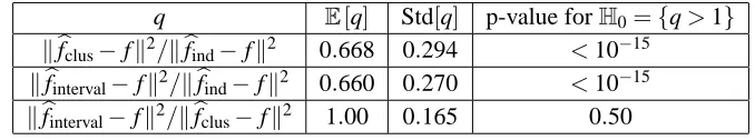
Experiments C–E are reported in Tables 1–3. The p-values correspond to the classical Gaussian difference test, where the hypotheses tested are of the shapeH₀₌_{_q_>₁_}_{against the hypotheses} H₁₌_{_q_≤₁_}_{, where the different quantities q are detailed in Tables 2–3.}

6.5 Comments

(17)

0 2 4 6 8 10 12 14 16 18 20 0.55

0.6 0.65 0.7 0.75 0.8 0.85 0.9 0.95 1

p

Ratio of the quadratic errors

With the estimated Σ

Figure 1: Increasing the number of tasks p (Experiment A), improvement of multi-task compared to single-task:E_[_kb_f

similar,bΣ−fk2/kfbind,Σb−fk2].

0 2 4 6 8 10 12 14 16 18 20

0 0.1 0.2 0.3 0.4 0.5 0.6 0.7 0.8 0.9

p

Quadratic errors, multi−task

With the estimated Σ With the true Σ

Figure 2: Increasing the number of tasks p (Experiment A), quadratic errors of multi-task estima-tors(np)−1_E_[_k_b_fsimilar,

(18)

0 2 4 6 8 10 12 14 16 18 20 0

0.1 0.2 0.3 0.4 0.5 0.6 0.7 0.8 0.9

p

Quadratic errors, single−task

Figure 3: Increasing the number of tasks p (Experiment A), quadratic errors of single-task estima-tors(np)−1_E_[_k_b_find,

S−fk2]. Blue: S=Σb. Red: S=Σ.

0 50 100 150

0 0.02 0.04 0.06 0.08 0.1 0.12 0.14 0.16

n

Figure 4: Increasing the sample size n (Experiment B), quadratic errors of multi-task estimators

(np)−1_E_[_k_b_fsimilar,

(19)

0 50 100 150 0

0.1 0.2 0.3 0.4 0.5 0.6 0.7 0.8

n

Quadratic errors, single−task

Figure 5: Increasing the sample size n (Experiment B), quadratic errors of single-task estimators

(np)−1_E_[_k_b_find,

S−fk2]. Blue: S=bΣ. Red: S=Σ.

0 50 100 150

0.4 0.5 0.6 0.7 0.8 0.9 1

n

Figure 6: Increasing the sample size n (Experiment B), improvement of multi-task compared to single-task:E_[_k_fb

(20)

0 2 4 6 8 10 12 0.02

0.04 0.06 0.08 0.1 0.12 0.14 0.16

Intensity of the noise matrix Σ

Figure 7: Increasing the signal-to-noise ratio (Experiment C), quadratic errors of multi-task estima-tors(np)−1_E_[_k_b_fsimilar,

S−fk2]. Blue: S=bΣ. Red: S=Σ.

0 2 4 6 8 10 12

0.4 0.5 0.6 0.7 0.8 0.9 1

Intensity of the noise matrix Σ

Figure 8: Increasing the signal-to-noise ratio (Experiment C), improvement of multi-task compared to single-task:E_[_kb_f

(21)

t 0.01 100

E_[_kb_f

similar,bΣ−fk2/kfbind,bΣ−fk2] 1.80±0.02 0.300±0.003 E_[_kb_f

similar,bΣ−fk2] (2.27±0.38)×10−2 0.357±0.048 E_[_kb_f_similar,_Σ₋_f_k2_] ₍₁_.₂₀_±₀_.₂₈₎_×₁₀−2 ₀_.₈₂₃_±₀_.₀₈₀

E_[_kb_f

ind,bΣ−fk2] (1.26±0.26)×10−2 1.51±0.07 E_[_kb_f_ind,_Σ₋_f_k2_] ₍₁_.₂₀_±₀_.₂₄₎_×₁₀−2 ₄_.₄₇_±₀_.₁₃

Table 1: Results of Experiment C for the extreme values of t.

q E_[_q_] _Std_[_q_] _{p-value for}H₀₌_{_q_>₁_}

kbfclus−fk2/kbfind−fk2 0.668 0.294 <10−15

kbfinterval₋f_k2/_kbfind₋f_k2 0.660 0.270 <10−15 kbfinterval−fk2/kbfclus−fk2 1.00 0.165 0.50

Table 2: Clustering and segmentation (Experiment D).

q n E_[_q_] _Std_[_q_] _{p-value for}H₀₌_{_q_>₁_}

kbf_similar,_Σ_b

HM−fk

2_/_k_b_fsimilar,CV₋_f_k2 ₁₀ ₀_.₃₅ ₀_.₄₆ _<₁₀−15

kbf_similar,_Σ_b

HM−fk

2_/_kb_f

similar,CV−fk2 50 0.56 0.42 <10−15

kbf_similar,_Σ_b

HM−fk

2_/_k_b_fsimilar,CV₋_f_k2 ₁₀₀ ₀_.₇₁ ₀_.₃₄ _<₁₀−15

kbf_similar,_Σ_b

HM−fk

2_/_k_b_f

similar,CV−fk2 250 0.87 0.19 <10−15

Table 3: Comparison of our method to 5-fold cross-validation (Experiment E).

A noticeable phenomenon also occurs in Figure 2 and even more in Figure 3: the estimator

b

find,Σ(that is, obtained knowing the true covariance matrixΣ) is less efficient than bf_ind,_b_Σ where the covariance matrix is estimated. It corresponds to the combination of two facts: (i) multiplying the ideal penalty by a small factor 1<Cn<1+o(1)is known to often improve performances in practice

when the sample size is small (see Section 6.3.2 of Arlot, 2009), and (ii) minimal penalty algorithms like Algorithm 14 are conjectured to overpenalize slightly when n is small or the noise-level is large (Lerasle, 2011) (as confirmed by Figure 7). Interestingly, this phenomenon is stronger for single-task estimators (differences are smaller in Figure 2) and disappears when n is large enough (Figure 5), which is consistent with the heuristic motivating multi-task learning: “increasing the number of tasks p amounts to increase the sample size”.

Figures 4 and 5 show that our procedure works well with small n, and that increasing n does not seem to significantly improve the performance of our estimators, except in the single-task setting withΣknown, where the over-penalization phenomenon discussed above disappears.

Table 2 shows that using the multitask procedure improves the estimation accuracy, both in the clustering setting and in the segmentation setting. The last line of Table 2 does not show that the clustering setting improves over the “segmentation into intervals” one, which was awaited if a model close to the oracle is selected in both cases.

(22)

7. Conclusion and Future Work

This paper shows that taking into account the unknown similarity between p regression tasks can be done optimally (Theorem 26). The crucial point is to estimate the p_×p covariance matrixΣ

of the noise (covariance between tasks), in order to learn the task similarity matrix M. Our main contributions are twofold. First, an estimator ofΣis defined in Section 4, where non-asymptotic bounds on its error are provided under mild assumptions on the mean of the sample (Theorem 20). Second, we show an oracle inequality (Theorem 26), more particularly with a simplified estimation ofΣand increased performances when the matrices of

M

are jointly diagonalizable (which often corresponds to cases where we have a prior knowledge of what the relations between the tasks would be). We do plan to expand our results to larger sets

M

, which may require new concentration inequalities and new optimization algorithms.

Simulation experiments show that our algorithm works with reasonable sample sizes, and that our multi-task estimator often performs much better than its single-task counterpart. Up to the best of our knowledge, a theoretical proof of this point remains an open problem that we intend to investigate in a future work.

Acknowledgments

This paper was supported by grants from the Agence Nationale de la Recherche (DETECTproject, reference ANR-09-JCJC-0027-01) and from the European Research Council (SIERRA Project ERC-239993).

We give in Appendix the proofs of the different results stated in Sections 2, 4 and 5. The proofs of our main results are contained in Sections E and F.

Appendix A. Proof of Proposition 8

Proof It is sufficient to show that_h·,_·iG is positive-definite on

G

. Take g∈

G

and S= (Si,j)1≤i≤j≤p

(23)

Let f be the element of

G

defined by∀i∈ {1. . .p}, g(_·,i) =∑n

k=1Ti,kf(·,k). We then have:

hg,g_iG=

p

∑

i=1 p

∑

j=1

Mi,jhg(·,i),g(·,j)iF

=

p

∑

i=1 p

∑

j=1 p

∑

k=1 p

∑

l=1

Mi,jTi,kTj,lhf(·,k),f(·,l)iF

=

p

∑

j=1 p

∑

k=1 p

∑

l=1

Tl,jhf(·,k),f(·,l)iF p

∑

i=1 Mj,iTi,k

=

p

∑

j=1 p

∑

k=1 p

∑

l=1

Tl,jhf(·,k),f(·,l)iF(M·T)j,k

=

p

∑

k=1 p

∑

l=1

Tl,jhf(·,k),f(·,l)iF p

∑

j=1

Tl,j(M·T)j,k

=

p

∑

k=1 p

∑

l=1

hf(_·,k),f(_·,l)_iF(T_·M_·T)k,l

=

p

∑

k=1

kf(_·,k)_k2

F.

This shows that_hg,g_iG _≥0 and that_hg,g_iG =0_⇒ f =0_⇒g=0.

Appendix B. Proof of Corollary 9

Proof If(x,j)_∈

X

× {1, . . . ,p_}, the application (f1, . . . ,fp)_7→ fj(x) is clearly continuous. We now show that(

G

,_h·,_·iG)is complete. If(gn)n∈N is a Cauchy sequence of

G

and if we define, as in Section A, the functions fnby∀n∈N,∀i∈ {1. . .p},gn(·,i) =∑_kp₌₁Ti,kfn(·,k). The same

com-putations show that(fn(·,i))n∈N are Cauchy sequences of

F

, and thus converge. So the sequence

(fn)n∈Nconverges in

G

, and(g_n)_n_∈Ndoes likewise.

Appendix C. Proof of Proposition 11

Proof We define

e

Φ(x,j) =M−1·

  

δ1,jΦ(x)

.. . δp,jΦ(x)

   ,

withδi,j=1i=jbeing the Kronecker symbol, that is,δi,j=1 if i=j and 0 otherwise. We now show

(24)

hg,Φe(x,l)_iG =

p

∑

j=1 p

∑

i=1

Mj,ihg(·,j),Φe(x,l)iiF

=

p

∑

j=1 p

∑

i=1 p

∑

m=1

Mj,iM_i−_,_m1δm,lhg(·,j),Φ(x)iF

=

p

∑

j=1 p

∑

m=1

(M_·M−1)j,mδm,lg(x,j)

=

p

∑

j=1

δj,lg(x,j) =g(x,l) .

Thus we can write:

ek((x,i),(y,j)) =_hΦe(x,i),Φe(y,j)_iG

=

p

∑

h=1 p

∑

h′₌₁

Mh,h′hM_h−_,1_iΦ(x),M_h−′1_,_jΦ(y)iF

=

p

∑

h=1 p

∑

h′₌₁

Mh,h′M_h−_,_i1M_h−_′_,1_jK(x,y)

=

p

∑

h=1

M−_h_,_i1(M·M−1)h,jK(x,y)

=

p

∑

h=1

M−_h_,_i1δh,jK(x,y) =Mi−,j1K(x,y) .

Appendix D. Computation of the Quadratic Risk in Example 12

We consider here that f1=_···= fp. We use the set

M

similar:

M

similar:=

Msimilar(λ,µ) = (λ+pµ)Ip− µ p11

⊤_/₍_λ_,µ₎_∈₍₀_,₊_∞₎2

Using the estimator bfM =AMy we can then compute the quadratic risk using the bias-variance

decomposition given in Equation (36):

E

bfM−f 2₂

=_k(AM−Inp)fk22+tr(A⊤MAM·(Σ⊗In)) .

Les us denote by(e1, . . . ,ep)the canonical basis ofRp. The eigenspaces of p−111⊤are: