Fast Approximate kNN Graph Construction for High Dimensional
Data via Recursive Lanczos Bisection
Jie Chen [email protected]
Department of Computer Science and Engineering University of Minnesota
Minneapolis, MN 55455, USA
Haw-ren Fang [email protected]
Mathematics and Computer Science Division Argonne National Laboratory
Argonne, IL 60439, USA
Yousef Saad [email protected]
Department of Computer Science and Engineering University of Minnesota
Minneapolis, MN 55455, USA
Editor: Sanjoy Dasgupta
Abstract
Nearest neighbor graphs are widely used in data mining and machine learning. A brute-force method to compute the exact kNN graph takesΘ(dn2)time for n data points in the d dimensional Euclidean space. We propose two divide and conquer methods for computing an approximate kNN graph inΘ(dnt)time for high dimensional data (large d). The exponent t∈(1,2)is an increasing function of an internal parameterαwhich governs the size of the common region in the divide step. Experiments show that a high quality graph can usually be obtained with small overlaps, that is, for small values of t. A few of the practical details of the algorithms are as follows. First, the divide step uses an inexpensive Lanczos procedure to perform recursive spectral bisection. After each conquer step, an additional refinement step is performed to improve the accuracy of the graph. Finally, a hash table is used to avoid repeating distance calculations during the divide and conquer process. The combination of these techniques is shown to yield quite effective algorithms for building kNN graphs.
Keywords: nearest neighbors graph, high dimensional data, divide and conquer, Lanczos
algo-rithm, spectral method
1. Introduction
Building nearest neighbor graphs is often a necessary step when dealing with problems arising from applications in such areas as data mining (Brito et al., 1997; Dasarathy, 2002), manifold learning (Belkin and Niyogi, 2003; Roweis and Saul, 2000; Saul and Roweis, 2003; Tenenbaum et al., 2000), robot motion planning (Choset et al., 2005), and computer graphics (Sankaranarayanan et al., 2007).
Given a set of n data points X={x1, . . . ,xn}, a nearest neighbor graph consists of the vertex set X
and an edge set which is a subset of X×X . The edges are defined based on a proximity measure
close. Two types of nearest neighbor graphs (Belkin and Niyogi, 2003; He and Niyogi, 2004) are often used:
1. ε-graph: This is an undirected graph whose edge set consists of pairs(xi,xj)such thatρ(xi,xj)
is less than some pre-defined thresholdε∈R+.
2. kNN graph: This is a directed graph (in general). There is an edge from xito xjif and only if
ρ(xi,xj)is among the k smallest elements of the set{ρ(xi,xℓ)|ℓ=1, . . . ,i−1,i+1, . . . ,n}.
Theε-graph is geometrically motivated, and many efficient algorithms have been proposed for
com-puting it (see, e.g., Bentley et al., 1977; Chazelle, 1983). However, theε-graph easily results in
dis-connected components (Belkin and Niyogi, 2003) and it is difficult to find a good value ofεwhich
yields graphs with an appropriate number of edges. Hence, they are not suitable in many situations. On the other hand, kNN graphs have been shown to be especially useful in practice. Therefore,
this paper will focus on the construction of kNN graphs, for the case whenρ(·,·)is the Euclidean
distance between two points in theRd.
When k=1, only the nearest neighbor for each data point is considered. This particular case,
the all nearest neighbors problem, has been extensively studied in the literature. To compute the 1NN graph, Bentley (1980) proposed a multidimensional divide-and-conquer method that takes
O(n logd−1n)time, Clarkson (1983) presented a randomized algorithm with expected O(cdn log n)
time (for some constant c), and Vaidya (1989) introduced a deterministic worst-case O((c′d)dn log n)
time algorithm (for some constant c′). These algorithms are generally adaptable to k>1. Thus,
Paredes et al. (2006) presented a method to build a kNN graph, which was empirically studied and reported to require O(n1.27)distance calculations for low dimensional data and O(n1.90)calculations for high dimensional data. Meanwhile, several parallel algorithms have also been developed (Calla-han, 1993; Callahan and Rao Kosaraju, 1995; Plaku and Kavraki, 2007). Despite a rich existing literature, efficient algorithms for high dimensional data are still under-explored. In this paper we propose two methods that are especially effective in dealing with high dimensional data.
Note that the problem of constructing a kNN graph is different from the problem of nearest
neighbor(s) search (see, e.g., Indyk, 2004; Shakhnarovich et al., 2006, and references therein),
where given a set of data points, the task is to find the k nearest points for any query point. Usually, the nearest neighbors search problem is handled by first building a data structure (such as a search tree) for the given points in a preprocessing phase. Then, queries can be answered efficiently by ex-ploiting the search structure. Of course, the construction of a kNN graph can be viewed as a nearest neighbors search problem where each data point itself is a query. However, existing search methods in general suffer from an unfavorable trade-off between the complexity of the search structure and the accuracy of the query retrieval: either the construction of the search structure is expensive, or accurate searches are costly. The spill-tree (sp-tree) data structure (Liu et al., 2004) is shown to be empirically effective in answering queries, but since some heuristics (such as the hybrid scheme) are introduced to ensure search accuracy, the construction time cost is difficult to theoretically
ana-lyze. On the other hand, many(1+ε)nearest neighbor search methods1have been proposed with
guaranteed complexity bounds (Indyk, 2004). These methods report a point within(1+ε)times the
distance from the query to the actual nearest neighbor. Kleinberg (1997) presented two algorithms.
The first one has a O((d log2d)(d+log n))query time complexity but requires a data structure of
size O(n log d)2d, whereas the second algorithm uses a nearly linear (to dn) data structure and
re-sponds to a query in O(n+d log3n)time. By using locality sensitive hashing, Indyk and Motwani
(1998) gave an algorithm that uses O(n1+1/(1+ε)+dn)preprocessing time and requires O(dn1/(1+ε))
query time. Another algorithm given in Indyk and Motwani (1998) is a O(d poly log(dn))search
al-gorithm that uses a O(n(1/ε)O(d)poly log(dn))data structure. Kushilevitza et al. (2000) proposed a
O((dn)2(n log(d log n/ε))O(ε−2)
poly(1/ε)poly log(dn/ε))data structure that can answer a query in
O(d2poly(1/ε)poly log(dn/ε))time. In general, most of the given bounds are theoretical, and have
an inverse dependence onε, indicating expensive costs when ε is small. Some of these methods
can potentially be applied for the purpose of efficient kNN graph construction, but many aspects,
such as appropriate choices of the parameters that controlε, need to be carefully considered before
a practically effective algorithm is derived. Considerations of this nature will not be explored in the present paper.
The rest of the paper is organized as follows. Section 2 proposes two methods for computing approximate kNN graphs, and Section 3 analyzes their time complexities. Then, we show a few ex-periments to demonstrate the effectiveness of the methods in Section 4, and discuss two applications in Section 5. Finally, conclusions are given in Section 6.
2. Divide and Conquer kNN
Our general framework for computing an approximate kNN graph is as follows: We divide the set of data points into subsets (possibly with overlaps), recursively compute the (approximate) kNN graphs for the subsets, then conquer the results into a final kNN graph. This divide and conquer framework can clearly be separated in two distinct sub-problems: how to divide and how to conquer. The conquer step is simple: If a data point belongs to more than one subsets, then its k nearest neighbors are selected from its neighbors in each subset. However, the divide step can be implemented in many different ways, resulting in different qualities of graphs. In what follows two methods are proposed which are based on a spectral bisection (Boley, 1998; Juhász and Mályusz, 1980; Tritchler et al., 2005) of the graph obtained from an inexpensive Lanczos procedure (Lanczos, 1950).
2.1 Spectral Bisection
Consider the data matrix
X= [x1, . . . ,xn]∈Rd×n
where each column xirepresents a data point inRd. When the context is clear, we will use the same
symbol X to also denote the set of data points. The data matrix X is centered to yield the matrix:
ˆ
X = [xˆ1, . . . ,xˆn] =X−ceT,
where c is the centroid and e is a column of all ones. A typical spectral bisection technique splits ˆX
into halves using a hyperplane. Let(σ,u,v)denote the largest singular triplet of ˆX with
uTXˆ =σvT. (1)
Then, the hyperplane is defined as hu,x−ci=0, that is, it splits the set of data points into two
subsets:
This hyperplane maximizes the sum of squared distances between the centered points ˆxi to the
hyperplane that passes through the centroid. This is because for any hyperplane hw,x−ci=0,
where w is a unit vector, the squared sum is
n
∑
i=1
(wTxˆi)2=
wTXˆ
2 2≤
Xˆ
2 2=σ
2,
while w=u achieves the equality.
By a standard property of the SVD (Equation 1), this bisection technique is equivalent to split-ting the set by the following criterion:
X+={xi|vi≥0} and X−={xi|vi<0}, (2)
where vi is the i-th entry of the right singular vector v. If it is preferred that the sizes of the two
subsets be balanced, an alternative is to replace the above criterion by
X+={xi|vi≥m(v)} and X−={xi|vi<m(v)}, (3)
where m(v)represents the median of the entries of v.
The largest singular triplet(σ,u,v)of ˆX can be computed using the Lanczos algorithm
(Lanc-zos, 1950; Berry, 1992). In short, we first compute an orthonormal basis of the Krylov subspace span{q1,(XˆTXˆ)q1, . . . ,(XˆTXˆ)s−1q1}for an arbitrary initial unit vector q1and a small integer s. Let
the basis vectors form an orthogonal matrix
Qs= [q1, . . . ,qs].
An equality resulting from this computation is
QTs(XˆTXˆ)Qs=Ts,
where Tsis a symmetric tridiagonal matrix of size s×s. Then we compute the largest eigenvalue
θ(s)and corresponding eigenvector y
sof Ts:
Tsys=θ(s)ys.
Therefore,θ(s)is an approximation to the square of the largest singular valueσ, while the vector
˜
vs≡Qsysis an approximation of the right singular vector v of ˆX . The acute angle∠(v˜s,v), between
˜
vsand v decays rapidly with s, as is shown in an error bound established in Saad (1980):
sin∠(v˜s,v)≤ K
Cs−1(1+γ1)
where K is a constant, Ck denotes the Chebyshev polynomial of degree k of the first kind, andγ1=
(λ1−λ2)/(λ2−λn)in which theλi’s denote the eigenvalues of ˆXTX , that is, the squared singularˆ
values of ˆX , ordered decreasingly. Note that we have Cs−1(1+γ1) =cosh[(s−1)cosh−1(1+γ1)],
in which cosh is the hyperbolic cosine. Therefore, a small value of s will generally suffice to yield an accurate approximation. Note that an exact singular vector is not needed to perform a bisection,
so we usually set a fixed value, say s=5, for this purpose. The computation of the orthonormal
basis takes timeΘ(sdn), while the time to computeθ(s)and y
sis negligible, since Tsis symmetric
tridiagonal and s is very small. Hence the time for computing the largest singular triplet of ˆX is
2.2 The Divide Step: Two Methods
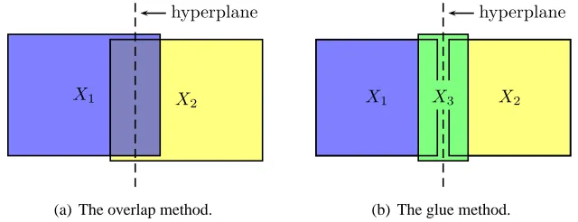
Based on the above general bisection technique, we propose two ways to perform the divide step for computing an approximate kNN graph. The first, called the overlap method, divides the current set into two overlapping subsets. The second, called the glue method, divides the current set into two disjoint subsets, and uses a third set called the gluing set to help merge the two resulting disjoint
kNN graphs in the conquer phase. See Figure 1. Both methods create a common region, whose size
is anα-portion of that of the current set, surrounding the dividing hyperplane. Details are given
next.
hyperplane
X1 X2
(a) The overlap method.
hyperplane
X1 X3 X2
(b) The glue method.
Figure 1: Two methods to divide a set X into subsets. The size of the common region in the middle
surrounding the hyperplane is anα-portion of the size of X .
2.2.1 THEOVERLAPMETHOD
In this method, we divide the set X into two overlapping subsets X1and X2:
(
X1∪X2=X, X1∩X26=/0.
Sinceσviis the signed distance from ˆxito the hyperplane, let the set V be defined as
V ={|vi| |i=1,2, . . . ,n}.
Then we use the following criterion to form X1and X2:
X1={xi|vi≥ −hα(V)} and X2={xi|vi<hα(V)}, (4)
where hα(·)is a function which returns the element that is only larger than(100α)% of the elements
in the input set. The purpose of criterion (4) is to ensure that the overlap of the two subsets consists of(100α)% of all the data, that is, that2
|X1∩X2|=⌈α|X|⌉.
2.2.2 THEGLUEMETHOD
In this method, we divide the set X into two disjoint subsets X1and X2with a gluing subset X3:
X1∪X2=X, X1∩X2=/0, X1∩X36=/0, X2∩X36=/0.
The criterion to build these subsets is as follows:
X1={xi|vi≥0}, X2={xi|vi<0}, X3={xi| −hα(V)≤vi<hα(V)}.
Note that the gluing subset X3 in this method is exactly the intersection of the two subsets in the
overlap method. Hence, X3also contains(100α)% of the data.
2.3 Refinement
In order to improve the quality of the resulting graph, during each recursion after the conquer step, the graph can be refined at a small cost. The idea is to update the k nearest neighbors for each point by selecting from a pool consisting of its neighbors and the neighbors of its neighbors. Formally,
if N(x) is the set of current nearest neighbors of x before refinement, then, for each point x, we
re-select its k nearest neighbors from
N(x)∪
[
z∈N(x)
N(z)
.
2.4 The Algorithms
We are ready to present the complete algorithms for both methods; see Algorithms 1 and 2. These algorithms share many similarities: They both fall in the framework of divide and conquer; they
both call the brute-force procedure kNN-BRUTEFORCE to compute the graph when the size of
the set is smaller than a threshold (nk); they both recursively call themselves on smaller subsets;
and they both employ a CONQUER procedure to merge the graphs computed for the subsets and
a REFINEprocedure to refine the graph during each recursion. The difference is that Algorithm 1
calls DIVIDE-OVERLAPto divide the set into two subsets (Section 2.2.1), while Algorithm 2 calls
DIVIDE-GLUEto divide the set into three subsets (Section 2.2.2). For the sake of completeness,
pseudocodes of all the mentioned procedures are given in Appendix A.
2.5 Storing Computed Distances in a Hash Table
The brute-force method computesΘ(n2) pairs of distances, each of which takesΘ(d) time. One
advantage of the methods presented in this paper over brute-force methods is that the distance cal-culations can be significantly reduced thanks to the divide and conquer approach. The distances
are needed/computed in: (1) the kNN-BRUTEFORCE procedure which computes all the pairwise
Algorithm 1 Approximate kNN Graph Construction: The Overlap Method
1: function G=kNN-OVERLAP(X , k,α)
2: if|X|<nk then
3: G←kNN-BRUTEFORCE(X , k)
4: else
5: (X1,X2)←DIVIDE-OVERLAP(X ,α) ⊲Section 2.2.1
6: G1←kNN-OVERLAP(X1, k,α)
7: G2←kNN-OVERLAP(X2, k,α)
8: G←CONQUER(G1, G2, k) ⊲Section 2, beginning
9: REFINE(G, k) ⊲Section 2.3
10: end if
11: end function
Algorithm 2 Approximate kNN Graph Construction: The Glue Method
1: function G=kNN-GLUE(X , k,α)
2: if|X|<nk then
3: G←kNN-BRUTEFORCE(X , k)
4: else
5: (X1,X2,X3)←DIVIDE-GLUE(X ,α) ⊲Section 2.2.2
6: G1←kNN-GLUE(X1, k,α)
7: G2←kNN-GLUE(X2, k,α)
8: G3←kNN-GLUE(X3, k,α)
9: G←CONQUER(G1, G2, G3, k) ⊲Section 2, beginning
10: REFINE(G, k) ⊲Section 2.3
11: end if
12: end function
k smallest distances from at most 2k candidates for each point, and (3) the REFINEprocedure which
selects the k smallest distances from at most k+k2 candidates for each point. Many of the
dis-tances computed from kNN-BRUTEFORCEand REFINEare reused in CONQUERand REFINE, with
probably more than once for some pairs. A naive way is to allocate memory for an n×n matrix
that stores all the computed distances to avoid duplicate calculations. However this consumes too much memory and is not necessary. A better approach is to use a hash table to store the computed distances. This will save a significant amount of memory, as a later experiment shows that only a
small portion of the n2 pairs are actually computed. Furthermore the computational time will not
be affected since hash tables are efficient for both retrieving wanted items from and inserting new items into the table (we do not need the delete operation).
The ideal hash function maps (the distance between) a pair of data points (xi,xj) to a bucket
such that the probability of collision is low. For simplicity of implementations, we use a hash
func-tion that maps the key(xi,xj)to i (and at the same time to j). Collisions easily occur since many
distances between the point xi and other points are computed during the whole process. However,
3. Complexity Analysis
A thorough analysis shows that the time complexities for the overlap method and the glue method are sub-quadratic (in n), and the glue method is always asymptotically faster than the overlap
method. To this end we assume that in each divide step the subsets X1and X2(in both methods) are
balanced. This assumption can always be satisfied by using the Equation (3) to bisect the data set,
instead of the criterion (2). Hence, the time complexity To for the overlap method and Tg for the
glue method satisfy the following recurrence relations:
To(n) =2To((1+α)n/2) +f(n), (5) Tg(n) =2Tg(n/2) +Tg(αn) +f(n), (6)
where f(n)is the combined time for the divide, conquer, and refine steps.
3.1 The Complexity of f
The function f(n)consists of the following three components.
3.1.1 THETIME FOR THEDIVIDESTEP
This includes the time to compute the largest right singular vector v of the centered matrix ˆX , and
the time to divide points into subsets X1and X2 (in the overlap method) or subsets X1, X2 and X3
(in the glue method). The former has been shown to be O(sdn)in Section 2.1, where the number
of Lanczos steps s=5 is fixed in the implementation, while for the latter we can use a linear time
selection method to find the value hα(V). Therefore the overall time for this step is O(dn).
3.1.2 THETIME FOR THECONQUER STEP
This step only involves the points in X1∩X2in the overlap method or X3in the glue method. For
each of theαn points in these subsets, k nearest neighbors are chosen from at most 2k candidates.
Therefore the time is O(kαn).
3.1.3 THETIME FOR THEREFINESTEP
For each point, k nearest neighbors are chosen from at most k+k2candidates. If all these distances
need to be computed, the overall time is O(k2dn). To the other extreme, if none of them are
com-puted, the factor d can be omitted, which results in O(k2n). In practice, by using a hash table, only
a very small fraction of the k+k2 distances are actually computed in this step; see also Table 3.
Hence, the best cost estimate for this step is O(k2n).
Indeed, the ultimate useful information from this estimate is that the time for the refinement is
much less than that for the division (which has a O(dn) cost), or at best is of the same order as
the latter. This can be seen from another perspective: Let the number of neighbors k be a constant.
Then even if all the distances are computed, the time is O(k2dn) =O(dn).
3.2 The Complexities of Toand Tg
By substituting f(n) =O(dn) into (5) and (6), we derive the closed form solutions to To(n) and
Tg(n), which are stated in the following two theorems.
Theorem 1 The time complexity for the overlap method is
To(n) =Θ(dnto),
where
to=log2/(1+α)2=
1
1−log2(1+α). Theorem 2 The time complexity for the glue method is
Tg(n) =Θ(dntg/α),
where tgis the solution to the equation
2
2t +α
t =1.
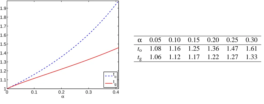
The proofs will be given in Appendix B. Figure 2 plots the two curves of toand tgas functions
ofα, together with a table that lists some of their values. Figure 2 suggests that the glue method is
asymptotically faster than the overlap method. Indeed, this is true for any choice ofα.
0 0.1 0.2 0.3 0.4
1 1.1 1.2 1.3 1.4 1.5 1.6 1.7 1.8 1.9
α
t
o
t
g
α 0.05 0.10 0.15 0.20 0.25 0.30
to 1.08 1.16 1.25 1.36 1.47 1.61 tg 1.06 1.12 1.17 1.22 1.27 1.33
Figure 2: The exponents toand tgas functions ofα.
Theorem 3 When 0<α<1, the exponents toin Theorem 1 and tgin Theorem 2 obey the following relation:
1<tg<to. (7)
The proof of the above theorem will be given in Appendix B. We remark that whenα>√2−
1≈0.41, to>2. In this situation the overlap method becomes asymptotically slower than the
brute-force method. Similarly, whenα>1/√2≈0.71, tg>2. Hence, a largeα(>0.41) is not useful in
4. Experiments
In this section we show a few experimental results to illustrate the running times of the two proposed methods compared with the brute-force method, and the qualities of the resulting graphs. The experiments were performed under a Linux workstation with two P4 3.20GHz CPUs and 2GB memory. The algorithms were all implemented using C/C++, and the programs were compiled using
g++with-O2level optimization. The divide and conquer methods were implemented according to
Algorithms 1 and 2, and the brute-force method was exactly as in the procedure kNN-BRUTEFORCE
given in Appendix A.
4.1 Running Time
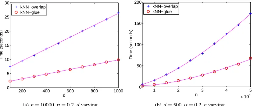
Figure 3 plots the running times versus the dimension d and the number of data points n on a syn-thetic data set. Since the distribution of the data should have little impact on the running times of
the methods, we used random data (drawn from the uniform distribution over[0,1]d) for this
exper-iment. From Figure 3(a), it is clear that the running time is linear with respect to the dimension d.
This is expected from the complexity analysis. In Figure 3(b), we usedα=0.2, which corresponds
to the theoretical values to=1.36 and tg=1.22. We used curves in the form c1n1.36+c2n+c3and
c4n1.22+c5n+c6to fit the running times of the overlap method and the glue method, respectively.
The fitted curves are also shown in Figure 3. It can be seen that the experimental results match the theoretical analysis quite well.
200 400 600 800 1000
0 5 10 15 20 25 30
d
Time (seconds)
kNN−overlap kNN−glue
(a) n=10000,α=0.2, d varying
1 2 3 4 5
x 104 0
50 100 150 200
n
Time (seconds)
kNN−overlap kNN−glue
(b) d=500,α=0.2, n varying
Figure 3: The running times for randomly generated data.
4.2 Quality
In another experiment, we used four real-life data sets to test the qualities of the resulting kNN
graphs: The FREY3face video frames (Roweis and Saul, 2000), the extYaleB4database (Lee et al.,
3. FREY can be found athttp://www.cs.toronto.edu/~roweis/data.html.
2005), the MNIST5 digit images (LeCun et al., 1998), and the PIE6 face database (Sim et al., 2003). These data sets are all image sets that are widely used in the literature in the areas of face recognition, dimensionality reduction, etc. For MNIST, we used only the test set. Table 1 gives some characteristics of the data. The number of images is equal to n and the size of each image, that is, the total number of pixels for each image, is the dimension d. The dimensions vary from
about 500 to 10,000. Since some of these data sets were also used later to illustrate the practical
usefulness of our methods in real applications, for each one we used a specific k value that was used in the experiments of past publications. These values are typically around 10.
FREY extYaleB MNIST PIE
# imgs (n) 1,965 2,414 10,000 11,554
img size (d) 20×28 84×96 28×28 32×32
Table 1: Image data sets.
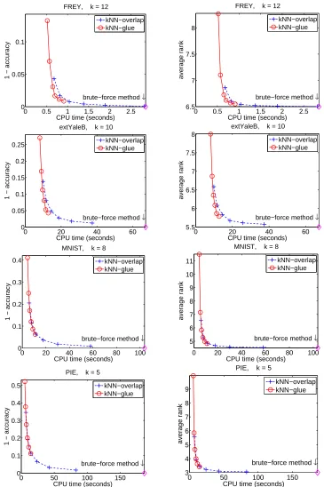
The qualities of the resulting graphs versus the running times are plotted in Figure 4. Each plotted point in the figure corresponds to a choice of α(=0.05,0.10,0.15,0.20,0.25,0.30). The running times of the brute-force method are also indicated. We use two quality criteria: accuracy
and average rank. The accuracy of an approximate kNN graph G′ (with regard to the exact graph
G) is defined as
accuracy(G′) =|E(G′)∩E(G)| |E(G)| ,
where E(·)means the set of directed edges in the graph. Thus, the accuracy is within the range
[0,1], and higher accuracy means better quality. The rank ru(v)of a vertex v with regard to a vertex
u is the position of v in the vertex list sorted in ascending order of the distance to u. (By default, the
rank of the nearest neighbor of u is 1.) Thus, the average rank is defined as
ave-rank(G′) = 1
kn
∑
u v∑
∈N(u)
ru(v),
where N(u)means the neighborhood of u in the graph G′. The exact kNN graph has the average
rank(1+k)/2.
It can be seen from Figure 4 that the qualities of the resulting graphs exhibit similar trends by
using both measures. Take the graph accuracy for example. The larger α, the more accurate the
resulting graph. However, larger values ofαlead to more time-consuming runs. In addition, the
glue method is much faster than the overlap method for the same α, while the latter yields more
accurate graphs than the former. The two methods are both significantly faster than the brute-force
method when an appropriate αis chosen, and they can yield high quality graphs even whenα is
small.
It is interesting to note that in all the plots, the red circle-curve and the blue plus-curve roughly overlap. This similar quality-time trade-off seems to suggest that neither of the method is superior
to the other one; the only difference is theαvalue used to achieve the desired quality. However,
we note that different approximate graphs can yield the same accuracy value or average rank value, hence the actual quality of the graph depends on real applications.
5. MNIST can be found athttp://yann.lecun.com/exdb/mnist.
0 0.5 1 1.5 2 2.5 0
0.05 0.1
FREY, k = 12
CPU time (seconds)
1 − accuracy
brute−force method ↓ kNN−overlap kNN−glue
0 0.5 1 1.5 2 2.5
6.5 7 7.5 8
FREY, k = 12
CPU time (seconds)
average rank
brute−force method ↓ kNN−overlap kNN−glue
0 20 40 60
0 0.05 0.1 0.15 0.2 0.25
extYaleB, k = 10
CPU time (seconds)
1 − accuracy
brute−force method ↓ kNN−overlap kNN−glue
0 20 40 60
5.5 6 6.5 7 7.5 8
extYaleB, k = 10
CPU time (seconds)
average rank
brute−force method ↓ kNN−overlap kNN−glue
0 20 40 60 80 100
0 0.1 0.2 0.3 0.4
MNIST, k = 8
CPU time (seconds)
1 − accuracy
brute−force method ↓ kNN−overlap kNN−glue
0 20 40 60 80 100
5 6 7 8 9 10 11
MNIST, k = 8
CPU time (seconds)
average rank
brute−force method ↓ kNN−overlap kNN−glue
0 50 100 150
0 0.1 0.2 0.3 0.4 0.5
PIE, k = 5
CPU time (seconds)
1 − accuracy
brute−force method ↓ kNN−overlap kNN−glue
0 50 100 150
3 4 5 6 7 8 9
PIE, k = 5
CPU time (seconds)
average rank
brute−force method ↓ kNN−overlap kNN−glue
Figure 4: Graph quality versus running time for different data sets. Each row of the plots
cor-responds to one data set. The left column of plots shows the 1−accuracy measure. The
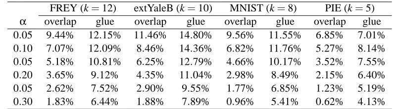
4.3 Distance Calculations and Refinements
We also report the percentage of the distance calculations, which is one of the dominant costs of the graph construction. The superior efficiency of our methods lies in two facts. First, for n data
points, the brute-force method must compute distances between n(n−1)/2 pairs of points, while
our methods compute only a small fraction of this number. Second, the use of a (hash) table brings the benefit of avoiding repeating distance calculations if the evaluations of the same distance are required multiple times. Tables 2 and 3 confirm these two claims. As expected, the larger the
common region (α) is, the more distances need to be calculated, while the benefit of the hashing
becomes more significant. It can also be seen that the savings in distance calculations are more
remarkable when n becomes larger and k becomes smaller, for example, k=5 for the data set PIE.
FREY (k=12) extYaleB (k=10) MNIST (k=8) PIE (k=5)
α overlap glue overlap glue overlap glue overlap glue
0.05 6.07% 5.10% 5.13% 4.42% 1.19% 0.94% 0.45% 0.35%
0.10 6.55% 5.80% 5.58% 5.08% 1.42% 1.22% 0.60% 0.47%
0.15 7.48% 6.35% 6.05% 5.46% 1.74% 1.36% 0.78% 0.56%
0.20 8.28% 6.57% 6.66% 5.66% 2.20% 1.52% 1.06% 0.66%
0.25 9.69% 7.00% 7.36% 6.02% 2.92% 1.71% 1.48% 0.77%
0.30 11.48% 7.46% 8.34% 6.26% 4.04% 1.91% 2.07% 0.90%
Table 2: Percentages of distance calculations (with respect to n(n−1)/2), for different data sets,
different methods, and differentα’s.
FREY (k=12) extYaleB (k=10) MNIST (k=8) PIE (k=5)
α overlap glue overlap glue overlap glue overlap glue
0.05 9.44% 12.15% 11.46% 14.80% 9.56% 11.55% 6.85% 7.01%
0.10 7.07% 12.09% 8.46% 14.36% 6.82% 11.76% 5.27% 8.14%
0.05 5.18% 10.81% 6.25% 12.79% 4.66% 10.17% 3.52% 7.55%
0.20 3.65% 9.12% 4.35% 11.04% 2.98% 8.49% 2.15% 6.40%
0.05 2.62% 7.52% 2.90% 9.55% 1.77% 6.85% 1.23% 5.19%
0.30 1.83% 6.44% 1.88% 7.89% 0.96% 5.41% 0.62% 4.13%
Table 3: Percentages of actual distance calculations with respect to the total number of needed
distances in the refine step, for different data sets, different methods, and different α’s.
This is equivalent to the failure rate of hash table lookups.
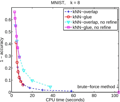
The final experiment illustrates the importance of the refine step. Figure 5 shows the decrease
in quality if the REFINEprocedure is not invoked. The refinement greatly improves the accuracy of
the approximate graph (especially forαless than 0.2) at some additional cost in the execution time.
This additional expense is worthwhile if the goal is to compute a high quality kNN graph.
5. Applications
kNN graphs have been widely used in various data mining and machine learning applications. This
0 20 40 60 80 100 0
0.1 0.2 0.3 0.4 0.5 0.6
MNIST, k = 8
CPU time (seconds)
1 − accuracy
brute−force method ↓ kNN−overlap
kNN−glue
kNN−overlap, no refine kNN−glue, no refine
Figure 5: The refine step boosts the accuracy of the graph at some additional computational cost. Data set: MNIST. The settings are the same as in Figure 4.
5.1 Agglomerative Clustering
Agglomerative clustering (Ward, 1963) is a clustering method which exploits a hierarchy for a set of data points. Initially each point belongs to a separate cluster. Then, the algorithm iteratively merges a pair of clusters that has the lowest merge cost, and updates the merge costs between the newly merged cluster and the rest of the clusters. This process terminates when the desired number of clusters is reached (or when all the points belong to the single final cluster). A straightforward
implementation of the method takes O(n3)time, since there are O(n)iterations, each of which takes
O(n2)time to find the pair with the lowest merge cost (Shanbehzadeh and Ogunbona, 1997). Fränti
et al. (2006) proposed, at each iteration, to maintain the kNN graph of the clusters, and merge two clusters that are the nearest neighbors in the graph. Let the number of clusters at the present iteration
be m. Then this method takes O(km)time to find the closest clusters, compared with the O(m2)cost
of finding the pair with the lowest merge cost. With a delicate implementation using a doubly linked
list, they showed that the overall running time of the clustering process reduces to O(τn log n), where
τis the number of nearest neighbor updates at each iteration. Their method greatly speeds up the
clustering process, while the clustering quality is not much degraded.
However, the quadratic time to create the initial kNN graph eclipses the improvement in the clustering time. One solution is to use an approximate kNN graph that can be inexpensively created. Virmajoki and Fränti (2004) proposed a divide-and-conquer algorithm to create an approximate
kNN graph, but their time complexity was overestimated. Our approach also follows the common
framework of divide and conquer. However, we bring three improvements over previous work: (1) Two methods to perform the divide step are proposed, (2) an efficient way to compute the separating hyperplane is described, and (3) a detailed and rigorous analysis on the time complexity is provided. This analysis in particular makes the proposed algorithms practical, especially in the presence of high dimensional data (e.g., when d is in the order of hundreds or thousands).
0.05 0.1 0.15 0.2 0.25 0.3 0.2 0.4 0.6 0.8 1
k = 5
α purity exact kNN kNN−overlap kNN−glue (a) Purity.
0.050 0.1 0.15 0.2 0.25 0.3
0.1 0.2 0.3 0.4
k = 5
α entropy exact kNN kNN−overlap kNN−glue (b) Entropy.
0.05 0.1 0.15 0.2 0.25 0.3
4.2 4.3 4.4 4.5 4.6 4.7x 10
5 k = 5
α
SSE
exact kNN kNN−overlap kNN−glue
(c) Sum of squared errors.
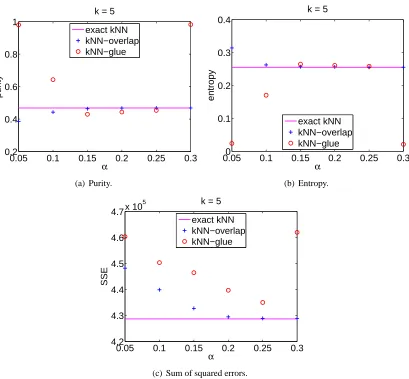
Figure 6: Agglomerative clustering using kNN graphs on the image data set PIE (68 human sub-jects).
They are defined as
Purity=
q
∑
i=1 ni
n Purity(i), where Purity(i) =
1
ni
max
j
nij
, and Entropy= q
∑
i=1 ni
nEntropy(i), where Entropy(i) =−
q
∑
j=1 nij ni
logqn
j i ni .
Here, q is the number of classes/clusters, ni is the size of cluster i, and nij is the number of class
j data that are assigned to the i-th cluster. The purity and the entropy both range from 0 to 1. In
Figure 6 we show the purities, the entropies, and the values of the objective function for a general
a higher purity, a lower entropy, and/or a lower SSE means a better clustering quality. As can be seen the qualities of the clusterings obtained from the approximate kNN graphs are very close to those resulting from the exact graph, with a few being even much better. It is interesting to note that the clustering results seem to have little correlation with the qualities of the graphs governed by the
valueα.
5.2 Dimensionality Reduction
Many dimensionality reduction methods, for example, locally linear embedding (LLE) (Roweis and Saul, 2000), Laplacian eigenmaps (Belkin and Niyogi, 2003), locality preserving projections (LPP) (He and Niyogi, 2004), and orthogonal neighborhood preserving projections (ONPP) (Kokiopoulou and Saad, 2007), compute a low dimensional embedding of the data by preserving the local neigh-borhoods for each point. For example, in LLE, a weighted adjacency matrix W is first computed to minimize the following objective:
E
(W) =∑
i
xi−∑xj∈N(xi)Wi jxj
2
, subject to
∑
j
Wi j=1,∀i,
where N(·)means the neighborhood of a point. Then, a low dimensional embedding Y= [y1, . . . ,yn]
is computed such that it minimizes the objective:
Φ(Y) =
∑
i
yi−∑yj∈N(yi)Wi jyj
2
, subject to YYT=I.
The final solution, Y , is the matrix whose column-vectors are the r bottom right singular vectors of
the Laplacian matrix LLLE=I−W . As another example, in Laplacian eigenmaps, the low
dimen-sional embedding Y = [y1, . . . ,yn]is computed so as to minimize the cost function:
Ψ(Y) =
∑
i,j Wi j
yi−yj
2
, subject to Y DYT=I,
where D is the diagonal degree matrix. Here, the weighted adjacency matrix W is defined in a number of ways, one of the most popular being the weights of the heat kernel
Wi j=
(
exp(−
xi−xj
2
/σ2) if x
i∈N(xj)or xj∈N(xi),
0 otherwise.
The solution, Y , is simply the matrix of r bottom eigenvectors of the normalized Laplacian matrix
Leigenmaps=I−D−1/2W D−1/2(subject to scaling).
A thorn in the nicely motivated formulations for the above approaches, is that they all begin with a rather expensive computation to obtain the neighborhood graph of the data. On the other hand, the cost of computing the solution Y via, for example, the Lanczos algorithm, is relatively
inexpensive, and can be summarized as7 O(rkn), which is independent of the dimension d. The
methods discussed in this paper are suitable alternatives to the expensive brute-force approach to
7. To be more exact, the dominant cost of computing r singular vectors/eigenvectors of a sparse matrix by the Lanczos
method is O(r′·nnz), where r′is the number of Lanczos steps and nnz is the number of nonzeros in the matrix. The
value r′is in practice a few times of r, and in our situation, the matrix is the (normalized) graph Laplacian, hence
−2 −1 0 1 2 3 4 −3
−2 −1 0 1 2 3 4
Using exact kNN
(a)
−2 −1 0 1 2 3 4
−3 −2 −1 0 1 2 3 4
Using kNN−overlap, α = 0.30
(b)
−1 −0.5 0 0.5 1 1.5 2 2.5
−3 −2 −1 0 1 2 3 4
Using kNN−glue, α = 0.15
(c)
−2 −1 0 1 2 3 4 5
−4 −3 −2 −1 0 1 2 3 4
Using kNN−glue, α = 0.30
(d)
(e) Images on the circle path. Facial expressions gradually change.
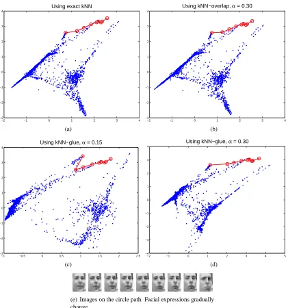
Figure 7: Dimensionality reduction on the data set FREY by LLE.
extract the exact kNN graph, since the approximate graphs are accurate enough for the purpose of dimensionality reduction, while the time costs are significantly smaller. Figures 7 and 8 provide two illustrations of this.
In Figure 7 are the plots of the dimensionality reduction results of LLE applied to the data set
FREY, where we used k=12 as that in Roweis and Saul (2000, Figure 3). Figure 7(a) shows
the result when using the exact kNN graph, while Figure 7(b) shows the result when using the
approximate kNN graph by the overlap method with α=0.30. It is clear that the two results are
−8 −6 −4 −2 0 2 4 6 8 x 10⁻³ −4
−2 0 2 4 6 8 10x 10
−3 Using exact kNN
0
1 2
3
4 5
6
7 8
9
(a)
−8 −6 −4 −2 0 2 4 6 8
x 10−3 −4
−2 0 2 4 6 8 10x 10
−3 Using kNN−overlap, α = 0.30
(b)
−8 −6 −4 −2 0 2 4 6
x 10−3 −4
−2 0 2 4 6 8 10x 10
−3 Using kNN−glue, α = 0.15
(c)
−8 −6 −4 −2 0 2 4 6
x 10−3 −4
−2 0 2 4 6 8 10x 10
−3 Using kNN−glue, α = 0.30
(d)
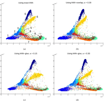
Figure 8: Dimensionality reduction on the data set MNIST by Laplacian eigenmaps.
embeddings are different from those of the exact kNN graph in Figure 7(a), they also represent the original data manifold quite well. This can be seen by tracking the relative locations of the sequence of images (as shown in 7(e)) in the two dimensional space.
Figure 8 shows the plots of the dimensionality reduction results of Laplacian eigenmaps applied
to the data set MNIST, where we used k=5. Figure 8(a) shows the original result by using the exact
kNN graph, while 8(b), 8(c) and 8(d) show the results by using the overlap method withα=0.30,
the glue method withα=0.15, and the glue method withα=0.30, respectively. The four plots
6. Conclusions
We have proposed two sub-quadratic time methods under the framework of divide and conquer for computing approximate kNN graphs for high dimensional data. The running times of the methods, as well as the qualities of the resulting graphs, depend on an internal parameter that controls the overlap size of the subsets in the divide step. Experiments show that in order to obtain a high quality graph, a small overlap size is usually sufficient and this leads to a small exponent in the time complexity. An avenue of future research is to theoretically analyze the quality of the resulting graphs in relation to the overlap size. The resulting approximate graphs have a wide range of applications as they can be safely used as alternatives to the exact kNN graph. We have shown two such examples: one in agglomerative clustering and the other in dimensionality reduction. Thus, replacing the exact kNN graph construction with one produced by the methods proposed here, can significantly alleviate what currently constitutes a major bottleneck in these applications.
Acknowledgments
This research was supported by the National Science Foundation (grant DMS-0810938) and by the Minnesota Supercomputer Institute. The authors would like to thank the anonymous referees who made many valuable suggestions.
Appendix A. Pseudocodes of Procedures
1: function G=kNN-BRUTEFORCE(X , k)
2: for i←1, . . . ,n do
3: for j←i+1, . . . ,n do
4: Computeρ(xi,xj) =
xi−xj
5: ρ(xj,xi) =ρ(xi,xj)
6: end for
7: Set N(xi) ={xj|ρ(xi,xj)is among the k smallest elements for all j6=i}
8: end for
9: end function
1: function(X1,X2) =DIVIDE-OVERLAP(X ,α)
2: Compute the largest right singular vector v of ˆX=X−ceT
3: Let V ={|vi| |i=1,2, . . . ,n}
4: Find hα(V) ⊲See Section 2.2.1 for the definition
5: Set X1={xi|vi≥ −hα(V)}
6: Set X2={xi|vi<hα(V)}
1: function(X1,X2,X3) =DIVIDE-GLUE(X ,α)
2: Compute the largest right singular vector v of ˆX=X−ceT
3: Let V ={|vi| |i=1,2, . . . ,n}
4: Find hα(V)
5: Set X1={xi|vi≥0}
6: Set X2={xi|vi<0}
7: Set X3={xi| −hα(V)≤vi<hα(V)}
8: end function
1: function G=CONQUER(G1, G2, k)
2: G=G1∪G2
3: for all x∈V(G1)∩V(G2)do ⊲V(·)denotes the vertex set of the graph
4: Update N(x)← {y|ρ(x,y)is among the k smallest elements for all y∈N(x)}
5: end for
6: end function
1: function G=CONQUER(G1, G2, G3, k)
2: G=G1∪G2∪G3
3: for all x∈V(G3)do
4: Update N(x)← {y|ρ(x,y)is among the k smallest elements for all y∈N(x)}
5: end for
6: end function
1: function REFINE(G, k)
2: for all x∈V(G)do
3: Update N(x)← {y|ρ(x,y)is among the k smallest elements for all
y∈N(x)∪S
z∈N(x)N(z)
}
4: end for
5: end function
Appendix B. Proofs
Theorem 1 follows from the Master Theorem (Cormen et al., 2001, Chapter 4.3). Theorem 2 is an immediate consequence of the following lemma, which is straightforward to verify.
Lemma 4 The recurrence relation
T(n) =2T(n/2) +T(αn) +n
with T(1) =1 has a solution
T(n) =
1+1
α
nt−n
α
where t is the solution to the equation
2
2t +α
t =1.
Lemma 5 When 0<x<1,
log2(1−x2)>log2(1−x)log2(1+x). Proof By Taylor expansion,
ln(1−x)ln(1+x)
= −
∞
∑
n=1 xn
n
! ∞
∑
n=1
(−1)n+1xn n
!
=−
∞
∑
n=1 2n−1
∑
m=1
(−1)m−1 m(2n−m)
!
x2n
=−
∞
∑
n=1
1 2n 1 1+ 1
2n−1
−2n1
1
2+
1
2n−2
+···+(−1)
n−1 n2
+··· − 1
2n
1
2n−2+
1 2 + 1 2n 1
2n−1+
1 1 x2n =− ∞
∑
n=1
1
n
1−1
2+
1
3+···+
1
2n−1
x2n
<−
∞
∑
n=1
ln 2
n
x2n
= (ln 2)·ln(1−x2).
The inequality in the lemma follows by changing the bases of the logarithms.
Lemma 6 The following inequality
log2(ab)>(log2a)(log2b)
holds whenever 0<a<1<b<2 and a+b≥2.
Proof By using b≥2−a, we have the following two inequalities
log2(ab)≥log2(a(2−a)) =log2(1−(1−a))(1+ (1−a)) =log2(1−(1−a)2)
and
(log2a)(log2b)≤(log2a)(log2(2−a)) =log2(1−(1−a))×log2(1+ (1−a)).
Then by applying Lemma 5 with 1−a=x, we have
log2(1−(1−a)2)>log2(1−(1−a))×log2(1+ (1−a)).
Proof of Theorem 3 From Theorem 2 we have
tg=1−log2(1−αtg)>1.
Then
to−tg=
1
1−log2(1+α)−1+log2(1−α
tg)
=log2(1+α) +log2(1−αtg)−log2(1+α)×log2(1−αtg)
1−log2(1+α) .
Since 0<α<1, the denominator 1−log2(1+α) is positive. By Lemma 6 the numerator is also
positive. Hence to>tg.
References
M. Belkin and P. Niyogi. Laplacian eigenmaps for dimensionality reduction and data representation.
Neural Computatioin, 16(6):1373–1396, 2003.
J. Bentley. Multidimensional divide-and-conquer. Communications of the ACM, 23:214–229, 1980.
J. Bentley, D. Stanat, and E. Williams. The complexity of finding fixed-radius near neighbors.
Information Processing Letters, 6:209–213, 1977.
M. W. Berry. Large scale sparse singular value computations. International Journal of
Supercom-puter Applications, 6(1):13–49, 1992.
D. L. Boley. Principal direction divisive partitioning. Data Mining and Knowledge Discovery, 2(4): 324–344, 1998.
M. Brito, E. Chávez, A. Quiroz, and J. Yukich. Connectivity of the mutual k-nearest neighbor graph in clustering and outlier detection. Statistics & Probability Letters, 35:33–42, 1997.
P. B. Callahan. Optimal parallel all-nearest-neighbors using the well-separated pair decomposition. In Proceedings of the 34th IEEE Symposium on Foundations of Computer Science, 1993.
P. B. Callahan and S. Rao Kosaraju. A decomposition of multidimensional point sets with appli-cations to k-nearest-neighbors and n-body potential fields. Journal of the ACM, 42(1):67–90, 1995.
B. Chazelle. An improved algorithm for the fixed-radius neighbor problem. Information Processing
Letters, 16:193–198, 1983.
H. Choset, K. M. Lynch, S. Hutchinson, G. Kantor, W. Burgard, L. E. Kavraki, and S. Thrun.
Principles of Robot Motion: Theory, Algorithms, and Implementations. The MIT Press, 2005.
K. L. Clarkson. Fast algorithms for the all nearest neighbors problem. In Proceedings of the 24th
T. H. Cormen, C. E. Leiserson, R. L. Rivest, and C. Stein. Introduction to Algorithms. The MIT Press, 2nd edition, 2001.
B. V. Dasarathy. Nearest-neighbor approaches. In Willi Klosgen, Jan M. Zytkow, and Jan Zyt, editors, Handbook of Data Mining and Knowledge Discovery, pages 88–298. Oxford University Press, 2002.
P. Fränti, O. Virmajoki, and V. Hautamäki. Fast agglomerative clustering using a k-nearest neighbor graph. IEEE Transactions on Pattern Analysis & Machine Intelligence, 28(11):1875–1881, 2006.
X. He and P. Niyogi. Locality preserving projections. In Advances in Neural Information Processing
Systems 16 (NIPS 2004), 2004.
P. Indyk. Nearest neighbors in high-dimensional spaces. In J. E. Goodman and J. O’Rourke, editors,
Handbook of Discrete and Computational Geometry. CRC Press LLC, 2nd edition, 2004.
P. Indyk and R. Motwani. Approximate nearest neighbors: towards removing the curse of dimen-sionality. In Proceedings of the Thirtieth Annual ACM Symposium on Theory of Computing, 1998.
F. Juhász and K. Mályusz. Problems of cluster analysis from the viewpoint of numerical analysis, volume 22 of Colloquia Mathematica Societatis Janos Bolyai. North-Holland, Amsterdam, 1980.
J. M. Kleinberg. Two algorithms for nearest-neighbor search in high dimensions. In Proceedings of
the Twenty-Ninth Annual ACM Symposium on Theory of Computing, 1997.
E. Kokiopoulou and Y. Saad. Orthogonal neighborhood preserving projections: A projection-based dimensionality reduction technique. IEEE Transactions on Pattern Analysis & Machine
Intelli-gence, 29(12):2143–2156, 2007.
E. Kushilevitza, R. Ostrovsky, and Y. Rabani. Efficient search for approximate nearest neighbor in high dimensional spaces. SIAM Journal on Computing, 30(2):457–474, 2000.
C. Lanczos. An iteration method for the solution of the eigenvalue problem of linear differential and integral operators. Journal of Research of the National Bureau of Standards, 45:255–282, 1950.
Y. LeCun, L. Bottou, Y. Bengio, and P. Haffner. Gradient-based learning applied to document recognition. Proceedings of the IEEE, 86(11):2278–2324, 1998.
K.C. Lee, J. Ho, and D. Kriegman. Acquiring linear subspaces for face recognition under variable lighting. IEEE Transactions on Pattern Analysis & Machine Intelligence, 27(5):684–698, 2005.
T. Liu, A. W. Moore, A. Gray, and K. Yang. An investigation of practical approximate nearest neighbor algorithms. In Proceedings of Neural Information Processing Systems (NIPS 2004), 2004.
R. Paredes, E. Chávez, K. Figueroa, and G. Navarro. Practical construction of k-nearest neighbor graphs in metric spaces. In Proceedings of the 5th Workshop on Efficient and Experimental
E. Plaku and L. E. Kavraki. Distributed computation of the knn graph for large high-dimensional point sets. Journal of Parallel and Distributed Computing, 67(3):346–359, 2007.
S. T. Roweis and L. K. Saul. Nonlinear dimensionality reduction by locally linear embedding.
Science, 290:2323–2326, 2000.
Y. Saad. On the rates of convergence of the Lanczos and the block-Lanczos methods. SIAM Journal
on Numerical Analysis, 17(5):687–706, 1980.
J. Sankaranarayanan, H. Samet, and A. Varshney. A fast all nearest neighbor algorithm for applica-tions involving large point-clouds. Computers and Graphics, 31(2):157–174, 2007.
L. K. Saul and S. T. Roweis. Think globally, fit locally: unsupervised learning of low dimensional manifolds. Journal of Machine Learning Research, 4:119–155, 2003.
G. Shakhnarovich, T. Darrell, and P. Indyk, editors. Nearest-Neighbor Methods in Learning and
Vision: Theory and Practice. The MIT Press, 2006.
J. Shanbehzadeh and P. O. Ogunbona. On the computational complexity of the LBG and PNN algorithms. IEEE Transactions on Image Processing, 6(4):614–616, 1997.
T. Sim, S. Baker, and M. Bsat. The CMU pose, illumination, and expression database. IEEE
Transactions on Pattern Analysis & Machine Intelligence, 25(12):1615–1618, 2003.
J. B. Tenenbaum, V. de Silva, and J. C. Langford. A global geometric framework for nonlinear dimensionality reduction. Science, 290(5500):2319–2323, 2000.
D. Tritchler, S. Fallah, and J. Beyene. A spectral clustering method for microarray data.
Computa-tional Statistics & Data Analysis, 49:63–76, 2005.
P. M. Vaidya. An O(n log n)algorithm for the all-nearest-neighbors problem. Discrete
Computa-tional Geometry, 4:101–115, 1989.
O. Virmajoki and P. Fränti. Divide-and-conquer algorithm for creating neighborhood graph for clus-tering. In Proceedings of the 17th International Conference on Pattern Recognition (ICPR’04), 2004.
J. H. Ward. Hierarchical grouping to optimize an objective function. Journal of the American
Statistical Association, 58(301):236–244, 1963.