Structure Spaces

Structure Spaces

Brijnesh J. Jain [email protected]

Klaus Obermayer [email protected]

Department of Electrical Engineering and Computer Science Berlin University of Technology

Berlin, Germany

Editor: Tommi Jaakkola

Abstract

Finite structures such as point patterns, strings, trees, and graphs occur as ”natural” representations of structured data in different application areas of machine learning. We develop the theory of structure spaces and derive geometrical and analytical concepts such as the angle between struc-tures and the derivative of functions on strucstruc-tures. In particular, we show that the gradient of a differentiable structural function is a well-defined structure pointing in the direction of steepest ascent. Exploiting the properties of structure spaces, it will turn out that a number of problems in structural pattern recognition such as central clustering or learning in structured output spaces can be formulated as optimization problems with cost functions that are locally Lipschitz. Hence, methods from nonsmooth analysis are applicable to optimize those cost functions.

Keywords: graphs, graph matching, learning in structured domains, nonsmooth optimization

1. Introduction

In pattern recognition and machine learning, it is common practice to represent data by feature vectors living in a Banach space, because this space provides powerful analytical techniques for data analysis, which are usually not available for other representations. A standard technique to solve a learning problem in a Banach space is to set up a smooth error function, which is then minimized by using local gradient information.

But often, the data we want to learn about have no natural representation as feature vectors and are more naturally represented in terms of finite combinatorial structures such as, for example, point patterns, strings, trees, lattices or graphs. Such learning problems arise in a variety of applications, which range from predicting the biological activity of a given chemical structure over finding fre-quent substructures of a data set of chemical compounds, and predicting the 3D-fold of a protein given its amino sequence, to natural language parsing, to name just a few.

distance spaces(

X

,d)of structures often have less mathematical structure than Banach spaces, sev-eral standard statistical pattern recognition techniques cannot be easily applied to(

X

,d).

There are two main approaches that apply standard statistical pattern recognition techniques to a given distance space(

X

,d). The first approach directly operates on the space(

X

,d). Examples are the k-nearest neighbor classifier, the linear programming machine (Graepel, Herbrich, Bollmann-Sdorra, and Obermayer, 1999), and pairwise clustering (Hofmann and Buhmann, 1997; Graepel and Obermayer, 1999). These methods can cope with sets

X

that possess an arbitrary distance function

d as the sole mathematical structure on

X

. The problem is that many pattern recognition methods require a space

X

with a richer mathematical structure. For example, large margin classifiers require as mathematical structure a complete vector space in which distances and angles can be measured. From an algorithmic point of view, many pattern recognition methods use local gradient information to minimize some cost function. For these methods, Banach spaces are endowed with enough structure to define derivatives and gradients.

The aim of the second approach is to overcome the lack of mathematical structure by embed-ding a given distance space (

X

,d) into a mathematically richer space (

X

′_,d′_{). Several methods}

have been proposed, which mainly differ in the choice of the target space

X

′ _{and to which}

ex-tent the original distance function d is preserved. Typical examples are embeddings into Euclidean spaces (Cox and Cox, 2000; Luo, Wilson, and Hancock, 2003; Minh and Hofmann, 2004), Hilbert spaces (G¨artner, 2003; Hochreiter and Obermayer, 2004, 2006; Kashima, Tsuda, and Inokuchi, 2003; Lodhi, Saunders, Shawe-Taylor, Cristianini, and Watkins, 2002), Banach spaces (Hein, Bous-quet, and Sch¨olkopf, 2005; von Luxburg and BousBous-quet, 2004), and Pseudo-Euclidean spaces (Her-brich, Graepel, Bollmann-Sdorra, and Obermayer, 1998; Goldfarb, 1985; Pekalska, Paclik, and Duin, 2001).

During this transformation, one has to ensure that the relevant information of the original prob-lem is preserved. Under the assumption that d is a reasonable distance function on

X

provided by some external knowledge, we can preserve the relevant information by isometrically embed-ding the original space (

X

,d) into some target space (

X

′_,d′_{). Depending on the choice of the}

target space this is only possible if the distance function d satisfies certain properties. Suppose that

S

=_{x1, . . . ,xk} ⊆

X

is a finite set and D= (di j)is a distance matrix with elements di j =d(xi,xj).

If d is symmetric and homogeneous, we can isometrically embed

D

into a Pseudo-Euclidean space (Goldfarb, 1985). In the case that d is a metric, the elements of

D

can be isometrically embedded into a Banach space. An isometric embedding of

S

into a Hilbert or Euclidean space is possible only if the matrix D2is of negative type (Schoenberg, 1937).1

Most standard learning methods have been developed in a Hilbert space or in a Euclidean space equipped with a Euclidean distance. But distance matrices of a finite set of combinatorial structures are often not of negative type and therefore an isometric embedding into a Hilbert space or Euclidean space is not possible. Another common problem of most isometric embeddings is that they only preserve distance relations and disregard knowledge about the inherent nature of the elements from the original space. For example the inherent nature of graphs is that they consist of a finite set of vertices together with a binary relation on that set. These information is lost, once we have settled in the target space for solving a pattern recognition problem. But for some methods in pattern recognition it is necessary to either directly access the original data or to recover the effects of the operations performed in the target space. One example is the sample mean of a set of combinatorial

structures (Jain and Obermayer, 2008; Jiang, M¨unger, and Bunke, 2001), which is a fundamental concept for several methods in pattern recognition such as principal component analysis and central clustering (Gold, Rangarajan, and Mjolsness, 1996; G¨unter and Bunke, 2002; Lozano and Escolano, 2003; Jain and Wysotzki, 2004; Bonev, Escolano, Lozano, Suau, Cazorla, and Aguilar, 2007; Jain and Obermayer, 2008). The sample mean of a set of vectors is the vector of sample means of each component of those vectors. Similarly, a sample mean of a set of combinatorial structures is a combinatorial structure composed of the sample means of the constituents parts the structure is composed of. Another example is finding frequent substructures in a given set of combinatorial structures (Dehaspe, Toivonen, and King, 1998; Yan and Han, 2002). For such problems a principled framework is missing.

In this contribution, we present a theoretical framework that isometrically and isostructurally embeds certain metric spaces(

X

,d)of combinatorial structures into a quotient space(

X

′,d′)of a Euclidean vector space. Instead of discarding information about the inherent nature of the original data, we can weaken the requirement that the embedding of(

X

,d)into(

X

′_,d′_{)should be isometric}

for all metrics. Here, we focus on metrics d that are related to the pointwise maximum of a set of Euclidean distances. This restriction is acceptable from an application point of view, because we can show that such metrics on combinatorial structures and their related similarity functions are a common choice of proximity measure in a number of different applications (Gold, Rangarajan, and Mjolsness, 1996; Holm and Sander, 1993; Caprara, Carr, Istrail, Lancia, and Walenz, 2004).

The quotient space(

X

′_,d′_{)preserves the distance relations and the nature of the original data.}

The related Euclidean space provides the mathematical structure that gives rise to a rich arsenal of learning methods. The goal of the proposed approach is to adopt standard learning methods based on local gradient information to learning on structures in the quotient space

X

′_{. In order to}

do so, we need an approach that allows us to formally adopt geometrical and analytical concepts for finite combinatorial structures. The proposed approach maps combinatorial structures to equiv-alence classes of vectors, where the elements of the same equivequiv-alence class are different vector representations of the same structure. Mapping a combinatorial structure to an equivalence class of vectors rather than to a single vector provides a link to the geometry of Euclidean spaces and at the same time preserves the nature of the original data. The resulting quotient set (the set of equiva-lence classes) leads to the more abstract notion of

T

-space. Formally, a

T

-space

X

T over a vector space

X

is a quotient set of

X

, where the equivalence classes are the orbits of the group action of a transformation group

T

on

X

. We show that

T

-spaces encompass a variety of different classes of combinatorial structures, which also includes vectors. Thus, the theory of

T

-spaces generalizes the vector space concept to cope with combinatorial structures and aims at retaining the geometrical and algebraic properties of a vector space to a certain extent.

We present case studies to illustrate that the theoretical framework can be applied to machine learning applications.

1/3

1/3 1/3 1/3 1/3

X₁ X₂ X₃ X−

1/3

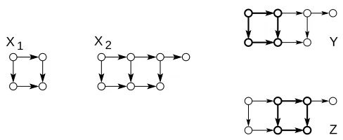
Figure 1: Illustration of a sample mean X of the three graphs

D

=_{X1,X2,X3}. Vertices and edges

of X that occur in all of the three example graphs from

D

are highlighted with bold lines. All other vertices and edges of X are annotated with the relative frequency of their occurrence in

D

. By annotating the highlighted vertices and edges of X with 1, we obtain a weighted graph.

problem of determining a sample mean of a set of structures including its application to central clustering. As structures we consider point patterns and attributed graphs. Section 6 concludes. Technical parts and proofs have been delegated to the appendix.

2. An Example

The purpose of this section is to provide an overview about the basic idea of the proposed approach. To this end, we consider the (open) problem of determining the sample mean of graphs as a sim-ple introductory examsim-ple. The concept of a samsim-ple mean is the theoretical foundation for central clustering algorithms (see Section 4.3 and references therein).

A directed graph is a pair X = (V,E) consisting of a finite set V of vertices and a set E =

{(i,j)_∈V_×V : i₆= j}of edges.

By

G

we denote the set of all directed graphs. Suppose that

D

= (X1, . . . ,Xk)

is a collection of k not necessarily distinct graphs from

G

. Our goal is to determine a sample mean of

X

. Intuitively, a sample mean averages the occurrences of vertices and edges within their structural context as illustrated in Figure 1.

As the sample mean of integers is not necessarily an integer, the sample mean of

D

is not necessarily a directed graph from

G

(see Figure 1). Therefore, we extend the set

G

of directed graphs to the set

G

[R] of weighted directed graphs. A weighted directed graph is a triple X= (V,E,α)consisting of a directed graph(V,E)and a weight functionα: V_∪V _→R_{such that each} edge has nonzero weight. A weighted directed graph X of order_|V_|=n is completely specified by

its weight matrix X= (xi j)with elements xi j=α(i,j)for all i,j∈ {1, . . . ,n}.

The standard method

X=1 k

k

∑

i=1 Xi

sum of squared Euclidean distances from the data points. In line with this formulation, we define a sample mean of

D

as a global minimum of the cost function

F(X) =

k

∑

i=1

D(X,Xi)2, (1)

where D is some appropriate distance function on

G

[R_{] that measures structural consistent and} inconsistent parts of the graphs under consideration.

In principle, we could use any ”well-behaved” distance function.2 Here, we first consider dis-tance functions on structures that generalize the Euclidean metric, because Euclidean spaces have a rich repository of analytical tools. To adapt at least parts of these tools for structure spaces, it seems to be reasonable to relate the distance function D in Equation (1) to the Euclidean metric. From an application point of view, this restriction is acceptable for the following reasons: (i) Geometric dis-tance functions on graphs and their related similarity functions are a common choice of proximity measure in a number of different applications (Gold, Rangarajan, and Mjolsness, 1996; Holm and Sander, 1993); and (ii) it can be shown that a number of structure-based proximity measures like, for example, the maximum common subgraph (Raymond and Willett, 2002) or maximum contact map overlap problem for protein structure comparison (Goldman, Istrail, and Papadimitriou, 1999) can be related to an inner product and therefore to the Euclidean distance.

The geometric distance functions D we consider here are usually defined as the maximum of a set of Euclidean distances. This definition implies that (i) the cost function F is neither differentiable nor convex; (ii) the sample mean of graphs is not unique as shown in Figure 2; and (iii) determining a sample mean of graphs is NP-complete, because evaluation of D is NP-complete. Thus, we are faced with an intractable combinatorial optimization problem, where, at a first glance, a solution has to be found from an uncountable infinite set. In addition, multiple local minima of the cost function

F complicates a characterization of a structural mean.

To deal with these difficulties, we embed graphs into a

T

-space as we will show shortly. The basic idea is to view graphs as equivalence classes of vectors via their weight matrices, where the elements of the same equivalence class are different vector representations of the same structure. The resulting quotient set (the set of equivalence classes) leads to the more abstract notion of

T

-space. Formally, a

T

-space

X

T over a vector space

X

is a quotient set of

X

, where the equivalence classes are the orbits of the group action of a transformation group

T

on

X

. The theory of

T

-spaces generalizes the vector space concept to cope with combinatorial structures and aims at retaining the geometrical and algebraic properties of a vector space to a certain extent. In doing so, the

T

-space concept not only clears the way to approach the structural version of the sample mean in a principled way, but also generalizes standard techniques of learning in structured domains.

2.1 The Basic Approach

To construct

T

-spaces, we demand that all graphs are of bounded order n, where the bound n can be chosen arbitrarily large. For a pattern recognition application this is not a serious restriction, because we can assume that the data graphs of interest are of bounded order. In the second step, we align each weighted directed graph X of order m<n to a graph X′of order n by adding p=n₋m

Z Y X₂

X₁

Figure 2: Illustration of one key problem in the domain of graphs: the lack of a well-defined ad-dition. The graph X1can be added to X2with respect to D(X1,X2)in two different ways

as indicated by the highlighted subgraphs of Y and Z. As a consequence, Y and Z can be regarded as two distinct sample means of X1and X2.

isolated vertices. The weighted adjacency matrix of the aligned graph X′ is then of the form

X′=

X 0m,p

0p,m 0p,p

,

where X is the weighted adjacency matrix of X , and 0m,p, 0p,m, 0p,pare padding zero matrices. By

G

[R_{,n]we denote the set of weighted directed graphs of bounded order n.}

For practical issues, it is important to note that restricting to structures of bounded order n and alignment of structures are purely technical assumptions to simplify mathematics. For machine learning problems, these limitations should have no practical impact, because neither the bound n needs to be specified nor an alignment of all graphs to an identical order needs to be performed. In a practical setting, we cancel out both technical assumptions by considering structure preserving mappings between the vertices of X and Y . Thus, when applying the theory, all we actually require is that the graphs are finite. We will return to this issue later, when we have provided the necessary technicalities.

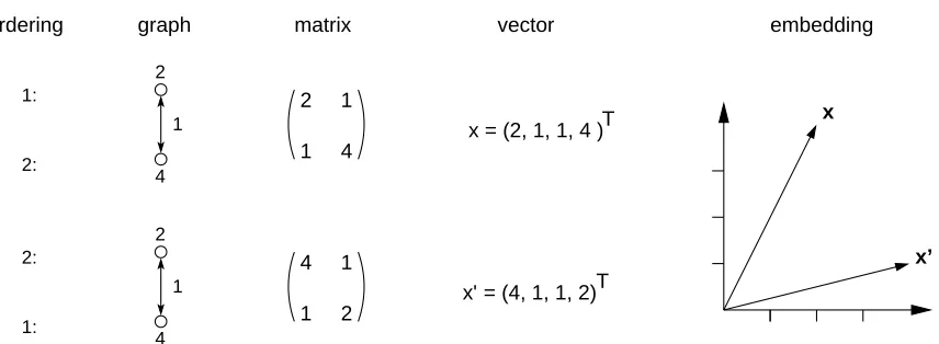
The positions of the diagonal elements of X determine an ordering of the vertices. Conversely, different orderings of the vertices may result in different matrices. Since we are interested in the structure of a graph, the ordering of its vertices does not really matter. Therefore, we consider two matrices X and X′as being equivalent, denoted by X_∼X′, if they can be obtained from one another by reordering the vertices. Mathematically, the equivalence relation can be written as

X_∼X′ _{⇔ ∃}P_∈

T

: PTX P=X′,

where

T

denotes the set of all(n_×n)-permutation matrices.3 The set

T

together with the function composition T_◦T′ for all T,T′ _∈

T

forms an algebraic group. By [X]we denote the equivalence class of all matrices equivalent to X . Occasionally, we also refer to[X]as the equivalence class of the graph X .

There are n! different orderings of the vertices for an arbitrary graph X with n vertices. Each of the n! orderings determines a weighted adjacency matrix. The equivalence class of X consist of all its different matrix representation. Note that different orderings of the vertices may result in the same matrix representation of the graph.

1 2 3 1 2 3 2 1 3 2 3 1 3 2 1 1 3 2 3 1 2 2 1 3 2 3 1 3 2 1 1 3 2 3 1 2 Y1 Y4

X1 X2 X5

Y6 Y2 X3 Y5 X6 Y3 X4

Figure 3: Illustration of two graphs with all possible orderings of their vertices. The number at-tached to the vertices represents their order (and are not attributes). The ordered graphs are grouped together according to their matrix representations. All ordered graphs X

1-X 6 yield the same weighted adjacency matrix. In the second row, the pairs (Y 1,Y 2),

(Y 3,Y 4), and(Y 5,Y 6)result in identical matrices.

Example 1 Consider the graphs X =X 1 and Y =Y 1 depicted in the first column of Figure 3. The numbers annotated to the vertices represent an arbitrarily chosen ordering. Suppose that all vertices and edges have attribute 1. Then the weighted adjacency matrices of X and Y given the chosen ordering of their vertices are of the form

X=





1 1 1 1 1 1 1 1 1



 and Y =





1 0 1 0 1 1 1 1 1





The first and second row of Figure 3 show the 3!=6 different orderings of X and Y , respectively.

The matrix representation of X is independent of its ordering, that is, each reordering of the vertices of X results in the same matrix representation. Hence, the equivalence class of X consists of the singleton X .

The 6 different orderings of graph Y result in three different matrix representations. The equiv-alence class of Y is of the form

[Y] =

  

 

1 0 1 0 1 1 1 1 1

 ,

 

1 1 1 1 1 0 1 0 1

 ,

 

1 1 0 1 1 1 0 1 1

 

  ,

where the first matrix refers to the ordering of Y =Y 1 and Y 2, the second to Y 3 and Y 4, and the third to Y 5 and Y 6.

Since we may regard matrices as vectors, we can embed X into the vector space

X

=Rn×n_as the set[X]of all vector representations of X . We call the quotient set

X

T =

X

/∼=

[

X∈X

[X]

2:

4

1 2 2:

1:

4 1:

1 2

T

1 4

x

x’

ordering graph matrix vector embedding

1 2

x’ = (4, 1, 1, 2) T 2 1

4 1

x = (2, 1, 1, 4 )

Figure 4: Illustration of an embedding of a graph of order 2. The attributes of the vertices are 2 and 4, and the attribute of the bidirectional edge is 1. Depending on the ordering of the vertices, we obtain two different matrix representations. Stacking the columns of the matrix to a 4-dimensional vector yields the vector representations x and x′. The plot in the last column depicts both representation vectors by considering their first and fourth dimension. Thus a graph is represented as a set of vectors in some vector space.

3.

T

-spaces

In this section, we formalize the ideas on

T

-spaces of the previous section. We consider a more general setting in the sense that we include classes of finite structures other than directed graphs with attributes from arbitrary vector spaces rather than weights fromR_{. The chosen approach that} allows to formally adopt geometrical and analytical concepts makes use of the notion of r-structures. We introduce r-structures in Section 3.1. Based on the notion of r-structures, we develop the theory of

T

-spaces in Sections 3.2 and 3.3. For a detailed technical treatment of

T

-spaces we refer to Appendix A and B. Finally, Section 3.4 considers optimization of locally Lipschitz functions on

T

spaces.

3.1 Attributed r-Structures

A r-structure is a pair X = (

P

,

R

) consisting of a finite set

P

6= /0, and a subset

R

⊆

P

r_{. The}

elements of

P

are the points of the r-structure X , the elements of

R

are its ary relations. A r-structure with points

P

is said to be a r-structure on

P

. For convenience, we occasionally identify the structure X on

P

with its relation

R

.

The following examples serve to indicate that several types of combinatorial structures can be regarded as r-structures. We first show that graphs are 2-structures. For this, we use the following notation: Given a finite set

P

of points, let

P

[2]=_{(p,q) : p,q_∈

P

,p₆=q_}

be the set of tuples from

P

2_{without diagonal elements(p,p).}

1. X is a directed graph if

R

⊆

P

[2]_.

2. X is a simple graph if

R

⊆

P

[2]_{such that(p,q)∈}

_R

_{implies(q,p)∈}

_R

_.

3. X is a simple graph with loops if

R

_⊆

P

2_{such that(p,q)∈}

_R

_{implies(q,p)∈}

_R

_{. Loops are} edges(p,p)with the same endpoints.

In a similar way, we can define further types of graphs such as, for example, trees, directed acyclic graphs, complete graphs, and regular graphs as 2-structures by specifying the corresponding properties on

R

.

The next example shows that elements of a set are 1-structures.

Example 3 (Set of Elements) Let

P

be a finite set of points. The elements E(

P

) = (

P

,

R

) is a

1-structure with

R

=

P

, that is its relations are the elements of

P

.

To introduce analytical concepts to functions on r-structures, we shift from discrete to contin-uous spaces by introducing attributes. Let

A

=

R

d _{denote the set of attributes. An}

_A

_-attributed

r-structure is a triple Xα = (

P

,

R

,α) consisting of a r-structure X = (

P

,

R

) and an attribution α:

P

r_→

_A

_{withα(p)6=0 if, and only if, p∈}

_R

_{. Besides the technical argument, attributions also}

have a practical relevance, because they are often used to enhance descriptions of structured objects. The next example collects some attributed structures.

Example 4 Let

P

be a finite set of order n.

• Attributed graphs: Let

A

=Rd_{. An attributed graph is an}

_A

_{-attributed 2-structure Gα}= (

P

,

R

,α), where G= (

P

,

R

)is a simple graph with loops andα:

R

_→

A

is an attribution that assigns each vertex (loop) and each edge a non-zero feature vector.

• Point patterns: Let

A

=R2_{. A point pattern is an}

_A

_{-attributed 1-structure Pα= (}

_P

_,

_R

,α_),

where E(

P

) = (

P

,

R

)are the elements of

P

andα:

R

→

A

is an attribution that assigns each element p_∈

P

its coordinatesα(p).

The next example shows that vectors are attributed 1-structures. Hence, all results on r-structures are also valid in vector spaces.

Example 5 Let

A

be a vector space. Suppose that

P

is of order n=1. A vector is an

A

-attributed

1-structure x_α= (

P

,

R

,α), where E(

P

) = (

P

,

R

) is the single element of

P

andα:

R

→

A

is an attribution that maps a singleton to a vector. Hence, the set of all possible structures xα on

P

reproduces the vector space

A

.

Note that we may assume without loss of generality that the attributes of r-relations from

R

are nonzero, that isα(

R

)_⊆

A

\ {0_}. If the zero vector 0 is required as a valid attribute of a r-relation, we can always change, for example, to the vector space

A

′₌

_A

_×R_{and redefine}α_as

α′_:

_P

r_→

_A

_{×R, p7→}

(0,0) : p_∈

P

r_\

_R

(α(p),1) : p_∈

R

.

An

A

-attributed r-structure X= (

P

,

R

,α)is completely specified by its matrix representation

X= (xp1...pr)with elements

for all p= (p1, . . . ,pr)∈

P

r. For example, the matrix representation of a simple graph is its ordinary

adjacency matrix.

Neither the ”nature” of the points

P

nor the particular form of the r-relations

R

of a given r-structure X = (

P

,

R

,α) do really matter. What matters is the structure described by

R

. Suppose that X is of order _|

P

_|=n. To abstract from the ”nature” of points, we chooseZ_{n={1, . . . ,n}as} our standard set of points. The particular form of

R

depends on the numbering of the points from Z_{n. To abstract from the particular form of}

_R

_{, we identify sets of r-relations that can be obtained}

from one another by renumbering the points. Mathematically, we can express these sets by means of isomorphism classes. Two

A

-attributed r-structures X = (

P

,

R

,α) and X′ = (

P

′,

R

′,α′) are

isomorphic, written as X_≃X′if there is a bijective mappingφ:

P

→

P

′_satisfying

1. p= (p1, . . . ,pr)∈

R

⇔ φ(p) = (φ(p1), . . . ,φ(pr))∈

R

′

2. α(p) =α′(φ(p))for all p_∈

R

.

The isomorphism class[X]of X consists of all

A

-attributed r-structures on

P

=Z_{nthat are} isomor-phic to X . By

S

_An,rwe denote the set of all

A

-attributed r-structures on

P

=Z_{nand by}

_S

n,r

A

the set of all isomorphism classes of structures from

S

_An,r.

We can identify any r-structure X = (Z_m,

_R

,α_{)of order m<n with a structure of order n by} adding q=n₋m isolated points. The aligned structure is then of the form X′= (Z_n,

_R

_,α′_{), where}

α′_{(p) =} α(p) : p∈

R

0 : otherwise .

Using alignment, we can regard

S

_An,r as the set of

A

-attributed r-structures of bounded order n. Similarly, we may think of

S

_An,ras the set of abstract

A

-attributed r-structures of bounded order

n. Again recall that specifying a bound n and aligning smaller structures to structures of order n are

purely technical assumptions to simplify mathematics.

3.2

T

-Spaces

Let

X

=Rn _{be the n-dimensional Euclidean vector space, and let}

_T

_{be a subgroup of the group of} all n_×n permutation matrices. Then the binary operation

·:

T

×

X

→

X

, (T,x)_7→T x

is a group action of

T

on

X

. For x∈

X

, the orbit of x is denoted by

[x]_T =_{T x : T _∈

T

}.

If no misunderstanding can occur, we write[x]instead of[x]_T.

A

T

-space over

X

is the orbit space

X

T =

X

/

T

of all orbits of x∈

X

under the action of

T

. We call

X

the representation space of

X

T. By

µ :

X

_→

X

T

we denote the membership function that sends vector representations to the structure they describe.

we can identify r-structures from

S

_An,r as vectors from

X

. Obviously, we have a relaxation in the sense that

S

_An,r_⊆

X

and

S

_An,r_⊆

X

T such that µ restricted on

S

An,rsends vector representations to the structures they represent. Note that there are structures in

X

T that are not well-defined r-structures from

S

_An,r. Hence, care must be taken when applying

T

-spaces.

The following notations, definitions, and results are useful to simplify technicalities. We use capital letters X,Y,Z, . . .to denote the elements of

X

T. Suppose that X=µ(x)for some x∈

X

. Then we identify X with[x]and make use of sloppy notations like, for example, x_∈X to denote x_∈[x].4

Let f :

X

_×

X

_→R_{be a symmetric function satisfying f(x,y) = f(y,x)for all x,y∈}

_X

_{. Then f} induces symmetric functions

F∗:

X

T ×

X

T →R, (X,Y)7→max{f(x,y): x∈X,y∈Y},

F_∗:

X

T ×

X

T →R, (X,Y)7→min{f(x,y) : x∈X,y∈Y}.

Since

T

is finite, the orbits[x]of x are finite. Hence, F∗and F_∗assume an extremal value. We call

F∗maximizer and F_∗minimizer of f on

X

T ×

X

T.

An inner product_h·,_·ion

X

gives rise to a maximizer of the form

h·,_·i∗:

X

T ×

X

T →R, (X,Y)7→max{hx,yi : x∈X,y∈Y}.

We call h·,_·i∗ inner

T

-product induced by h·,_·i. The inner

T

-product is not an inner product, because the maximum-operator in the definition of_h·,_·i∗does not preserve the bilinearity property of an inner product. But we can show that an inner

T

-product satisfies some weaker properties.

1 3

1 1 2

4

3 1

1 1

1 1

1 3

embedding

x

x’ y’

y x = (2, 1, 1, 4) T

x’ = (4, 1, 1, 2)

y = (3, 1, 1, 1) T

y’ = (1, 1, 1, 3) T

matrices vectors

graphs

Y

T 2 1

1 4

4 1

1 2 X

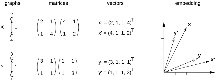
Figure 5: Illustration of two example graphs and their embeddings in a vector space (see Figure 4 for a detailed description).

Example 6 Consider the graphs X and Y from Figure 5. We have

hX,Y_i∗=x,y′=x′,y=16.

4. The notation is sloppy, because X is an element inX_T and not a set, whereas[x]is a set of equivalent elements from

Thus, to determine hX,Yi∗, we select vector representations ˜x of X and ˜y of Y that have closest angle and then evaluate_hx˜,y˜_i.

Any inner product space

X

is a normed space with norm_kx_k=p_hx,x_iand a metric space with metric d(x,y) =_kx₋y_k. The norm_k·kand the metric d on

X

give rise to minimizers_k·k∗ of_k·k and D_∗of d on

X

T.

Since elements from

T

preserve lengths and angles, we have

kT x_k=_kT x₋0_k=_kT x₋T 0_k=_kx₋0_k=_kx_k

for all T _∈

T

. Hence,_kX_k∗ is independent from the choice of vector representation. We call the minimizer_k·k∗the

T

-norm induced by the norm_k·k. A

T

-norm is related to an inner

T

-product in the same way as a norm to an inner product. We have

1. _hX,X_i∗=_hx,x_ifor all x_∈X .

2. _kX_k∗=p_hX,X_i∗.

Note that a

T

-norm is not a norm, because a

T

-space has no well defined addition. But we can show that a

T

-norm has norm-like properties.

Example 7 Consider the graphs X and Y from Figure 5. To determine their

T

-norm, it is sufficient to compute the standard norm of an arbitrarily chosen vector representation. Hence, we have

kX_k∗=_kx_k=x′=√22, kY_k∗=_ky_k=y′=√12.

The minimizer D_∗of the Euclidean metric d(x,y) =_kx₋y_kis also a metric. To distinguish from ordinary metrics, we call the minimizer D_∗ of a Euclidean metric d on

X

the

T

-metric induced by

d. We can express the metric D_∗in terms ofh·,_·i∗as follows:

D_∗(X,Y)2=_kX_k2_∗−2_hX,Y_i∗+_kY_k2_∗.

Example 8 Consider the graphs X and Y depicted in Figure 5. To determine D_∗(X,Y), we select vector representations ˜x of X and ˜y of Y that have minimal distance d(x˜,y˜). Then we find that

D_∗(X,Y) =d(x,y′) =d(x′,y) =√2.

3.3 Functions on

T

-Spaces

A

T

-function is a function of the form

F :

X

T →R,

where

X

T is a T -space over

X

. Instead of considering the

T

-function F, it is often more convenient to consider its representation function

which is invariant under transformations from elements of

T

.

Here, the focus is on

T

-functions that are locally Lipschitz. A

T

-function is locally Lipschitz if, and only if, its representation function is locally Lipschitz. We refer to Appendix C for basic definitions and properties from nonsmooth analysis of locally Lipschitz functions.

Suppose that F is a locally Lipschitz function with representation function f . By Rademacher’s Theorem 23, f is differentiable almost everywhere. In addition, at non-differentiable points, f admits the concept of generalized gradient. The concepts differentiability and gradient can be trans-fered to

T

-spaces in a well-defined way. Assume that f is differentiable at some point x_∈

X

with gradient∇f(x). Then f is differentiable at all points T x_∈X with T _∈

T

and the gradient of f at T x is of the form

∇f(T x) =T∇f(x).

We say F is

T

-differentiable at X , if its representation function f is differentiable at an arbitrary vector representation x_∈X . The well-defined structure

∇F(X) =µ(f(x))

is the

T

-gradient of F at X pointing in direction of steepest ascent.

3.4 Optimization of Locally Lipschitz

T

-Functions

A standard technique in machine learning and pattern recognition is to pose a learning problem as an optimization problem. Here, we consider the problem of solving optimization problems of the form

(P1) minimize F :

X

T →R, X7→∑

k

i=1Fi(X)

subject to X∈

U

T

where the component functions Fi are locally Lipschitz

T

-functions and

U

T ⊂

X

T is the feasible set of admissible solutions. Then according to Prop. 21, the cost function F is also locally Lipschitz, and we can rewrite (P1) to an equivalent optimization problem

(P2) minimize f :

X

→R, x7→∑

k i=1fi(x)

subject to x_∈

U

where the component functions fiare the representation functions of Fi and

U

⊆

X

is the feasible

set with µ(

U

) =

U

T. Hence, f is the representation function of the locally Lipschitz

T

-function F and therefore also locally Lipschitz.

Algorithm 1 (Basic Incremental Algorithm)

choose starting point x1∈U and set t :=0

repeat

set ˜xt,1:=x1

for i=1, . . . ,k do

direction finding:

determine d_t,i∈X andη>0 s.t. ˜x_t,i+ηd_t,i∈Uand

fi(x˜t,i+ηdt,i)<fi(x˜t,i)

line search:

find step sizeηt,i>0 such that ˜xt,i+ηt,idt,i∈Uand

ηt,i≈arg min_η

>0fi(x˜t,i+ηdt,i)

updating:

set ˜xt,i+1:=x˜t,i+ηt,idt,i Set xt+1:=x˜t,k+1

Set t :=t+1

until some termination criterion is satisfied

To explain the algorithm, we first consider the case that f is smooth and

U

=

X

. In the step

direction finding, we generate a descent direction by exploiting the fact that the direction opposite

to the gradient is locally the steepest descent direction. Line search usually employs some efficient univariate smooth optimization method or polynomial interpolation. The necessary condition for a local minimum yields a termination criterion. Now suppose that f is locally Lipschitz. Then f admits a generalized gradient at each point. The generalized gradient coincides with the gradient at differentiable points and is a convex set of subgradients at non-differentiable points. For more details, we refer to Appendix C.

Subgradients, the elements of a generalized gradient, play a very important role in algorithms for non-differentiable optimization. The basic idea of subgradient methods is to generalize the methods for smooth problems by replacing the gradient by an arbitrary subgradient. In the direction finding step, Algorithm 1 computes an arbitrary subgradient d_∈∂f(x) at the current point x. If

f is differentiable at x, then the subgradient d coincides with the gradient ∇f(x). If in addition

d₆=0, then the opposite direction₋d is the direction of steepest descent. On the other hand, if f

is not differentiable at x, then₋d is not necessarily a direction of descent of f at x. But since f is

differentiable almost everywhere by Rademacher’s Theorem 23, the set of non-differentiable points is a set of Lebesgue measure zero.

Line search uses predetermined step sizesηt,i, instead of an exact or approximate line search

as in the gradient method. One reason for this is that the direction₋d computed in the direction

finding step is not necessarily a direction of descent. Thus, the viability of subgradient methods depend critically on the sequence of step sizes. One common choice are step sizes that satisfy

∞

∑

t=0

ηt=∞ and

∞

∑

t=0

whereηt=ηt,1.

To formulate a termination criterion, we could—in principle—make use of the following nec-essary condition of optimality.

Theorem 1 Let f :

X

→R_{be locally Lipschitz at its minimum (maximum) x∈}

_R

_{. Then}

0_∈∂f(x).

At non-differentiable points, however, an arbitrary subgradient provides no information about the existence of the zero in the generalized gradient ∂f(x). Therefore, when assuming an instantly decreasing step size, one reliable termination criterion stops the algorithm as soon as the step size falls below a predefined threshold.

Since the subgradient method is not a descent method, it is common to keep track of the best point found so far, which is the one with smallest function value. For further advanced and more so-phisticated techniques to minimize locally Lipschitz functions, we refer to M¨akel¨a and Neittaanm¨aki (1992); Shor (1985).

We conclude this section with a remark on determining intractable subgradients in a practical setting.

3.4.1 APPROXIMATINGSUBGRADIENTS

Nonsmooth optimization as discussed in M¨akel¨a and Neittaanm¨aki (1992); Shor (1985) assumes that at each point x we can evaluate at least one subgradient y_∈∂f(x)and the function value f(x). In principle, this should be no obstacle for the class of problems we are interested in. In a practical setting, however, evaluating a subgradient as descent direction can be computationally intractable. For example, the pattern recognition problems described later in Section 4.2-4.5 are all computa-tionally efficient for structures like point patterns, but NP-hard for structures like graphs. A solution to this problem is to approximate a subgradient by using polynomial time algorithms. An approx-imated subgradient corresponds to a direction that is no longer a subgradient of the cost function. In particular, at smooth points, an approximated (sub)gradient (hopefully) corresponds to a descent direction close to the direction of steepest descent. We call Algorithm 1 an approximate

incremen-tal subgradient methods if the direction finding step produces directions that are not necessarily

subgradients of the corresponding component function fi.

We replace the subgradient by a computationally cheaper approximation as a direction of de-scent. In a computer simulation, we show that determining a sample mean of weighted graph is indeed possible when using approximate subgradient methods.

Suppose that

X

T is the

T

-space of simple weighted graphs over

X

=Rn×n, and let

U

T ⊆

X

T be the subset of weighted graphs with attributes from the interval[0,1]. Our goal is to determine a sample mean of a collection of simple weighted graphs

D

=_{

X1

, . . . ,

X

k} ⊆

U

T.

Given a representation x of X , the computationally intractable task is to find a representation xi

of Xi such that(x,xi)∈supp dX2i|x

. This problem is closely related to the problem of computing the distance D_∗(X,Xi), which is known to be an NP-complete graph matching problem. Hence,

descent. We call Algorithm 1 an approximate incremental subgradient methods if the direction find-ing step produces directions that are not necessarily subgradients of the correspondfind-ing component function fi.

4. Pattern Recognition in

T

-Spaces

This section shows how the framework of

T

-spaces can be applied to solve problems in structural pattern recognition. We first propose a generic scheme for learning in distance spaces. Based on this generic scheme, we derive cost functions for determining a sample mean, central clustering, learning large margin classifiers, supervised learning in structured input and/or output spaces, and finding frequent substructures. Apart from the last problem, all other cost functions presented in this section extend standard cost functions from the vector space formalism to

T

-spaces in the sense that we recover the standard formulations when regarding vectors as r-structures.

4.1 A Generic Approach: Learning in Distance Spaces

Without loss of generality, we may assume that (

X

T,D) is a distance space, where D is either the metric D_∗ induced by the Euclidean metric on

X

or another (not necessarily metric) distance function that is more appropriate for the problem to hand. A generic approach to solve a learning problem(P)in

X

T is as follows:

1. Transform(P)to an optimization problem, where the cost function F is a function defined on

X

T.

2. Show that F is locally Lipschitz.

3. Optimize F using methods from nonsmooth optimization.

Since

X

T is a metric space over an Euclidean vector space, we can apply subgradient methods or other techniques from nonsmooth optimization to minimize locally Lipschitz

T

-functions on

X

T. If the cost function F depends on a distance measure D, we demand that D is locally Lipschitz to ensure the locally Lipschitz property for F.

4.2 The Sample Mean of k-Structures

The sample mean of structures is a basic concept for a number of methods in statistical pattern recognition. Examples include visualizing or comparing two populations of chemical graphs, and central clustering of structures (Section 4.3).

We define a sample mean of the k elements X1, . . . ,Xk∈

X

T as a minimizer of minimize F(X) =∑k

i=1D(X,Xi)2

subject to X_∈

X

T

,

where D is a distance function on

X

T. If D is locally Lipschitz, then F is also locally Lipschitz by Prop. 21.

function, they applied a genetic algorithm to graphs with a small number of discrete attributes. In this contribution, we shift the problem of determining a sample mean from discrete to continuous optimization.

4.3 Central Clustering of k-Structures

Suppose that we are given a training sample

X

=_{X1, . . . ,Xm}consisting of m structures Xidrawn

from the structure space

X

T. The aim of central clustering is to find k cluster centers

Y

={Y1, . . . ,Yk}

⊆

X

T such that the following cost function

F(M,

Y

,

X

) = 1 m

k

∑

j=1 m

∑

i=1

mi jD(Xi,Yj),

is minimized with respect to a given distortion measure D. The matrix M= (mi j) is a (m×k)

-membership matrix with elements mi j∈[0,1]such that∑jmi j=1 for all i=1, . . . ,m.

If the distortion measure is locally Lipschitz, then F as a function of the cluster centers Yj is

locally Lipschitz by Prop. 21.

A number of central clustering algorithms for graphs have been devised recently (Gold, Ran-garajan, and Mjolsness, 1996; G¨unter and Bunke, 2002; Lozano and Escolano, 2003; Jain and Wysotzki, 2004; Bonev, Escolano, Lozano, Suau, Cazorla, and Aguilar, 2007). In experiments it has been shown that the proposed methods converge to satisfactory solutions, although neither the notion of cluster center nor the update rule of the cluster centers is well-defined. Because of these issues one might expect that central clustering algorithm could be prone to oscillations halfway be-tween different cluster centers of the same cluster. An explanation why this rarely occurs can now be given. As long as the cost function is locally Lipschitz, almost all points are differentiable. For these points the update rule is well-defined. Hence, it is very unlikely that the aforementioned oscil-lations occur over a longer period of time, when using an optimization algorithm that successively decreases the step size.

4.4 Large Margin Classifiers

Consider the function

hW,b:

X

T →R, X7→ hW,Xi∗+b,

where W _∈

X

T is the weight structure and b∈R the bias. The discriminant hW,b implements a

two-category classifier in the obvious way: Assign an input structure X to the class labeled+1 if

hW,b(X)≥0 and to−1 if hW,b(X)<0.

Suppose that

Z

=_{(X1,y1), . . . ,(Xk,yk)}is a training sample consisting of k training structures

Xi∈

X

T together with corresponding labels yi∈ {±1}. We say,

Z

is

T

-separable if there exists a

W0∈

X

T and b0∈Rwith

h_∗(X) =_hW0,Xi∗+b0=y

for all(X,y)_∈

Z

.

To find an ”optimal” discriminant that correctly classifies the training examples, we construct the cost function

F(W,b,α) =1

2kWk

2 ∗−

k

∑

i=1

where theαi≥0 are the Lagrangian multipliers. The representation function of F is of the form

f(w,b,α) =1

2kwk

2

−

k

∑

i=1

αiyi(si(w,b)−1),

where si(w,b) =maxT_∈Thw,T xii+b. The elements w∈W and xi∈Xiare arbitrary. The first term

of f is smooth and convex (and therefore locally Lipschitz). The locally Lipschitz property and convexity of the second term follows from the rules of calculus for locally Lipschitz functions (see Section C) and Prop. 20. Hence, f is locally Lipschitz and convex.

The structurally linear discriminants sets the stage to (i) explore large margin classifiers in struc-ture spaces and (ii) construct neural learning machines for adaptive processing of finite strucstruc-tures. Subgradient methods for maximum margin learning has been applied in Ratliff, Bagnell, and Zinke-vich (2006) for predicting structures rather than classes. Finally note that the inner

T

-product as a maximizer of a set of similarities is not a kernel (G¨artner, 2005).

4.5 Supervised Learning

The next application example generalizes the problem of learning large margin classifiers for k-structures by allowing

T

-spaces as input and as output space. Note that the in- and output spaces may consist of different classes of k-structures, for example, the input patterns can be feature vectors and the output space can be the domain of graphs.

Assume that we are given a a training sample

Z

=_{(X1,Y1), . . . ,(Xk,Yk)}consisting of k training

structures Xidrawn from some

T

-space

X

T over

X

together with corresponding output structures Yi

from a

T

′_-space

_Y

T′ over

Y

. Given the training data

Z

, our goal is to find an unknown functional relationship (hypothesis)

H :

X

T →

Y

T

from a hypothesis space

H

that best predicts the output structures of unseen examples (X,Y)_∈

X

T ×

Y

T according to some cost function

F(H,

Z

) =1 k

k

∑

i=1

L(H(Xi),Yi),

where L :

Y

T ×

Y

T →Rdenotes the loss function. The representation function of F is of the form

f(h,

Z

) =1 k

k

∑

i=1

ℓ(h(xi),yi),

whereℓ:

Y

×

Y

→R_{is the representation function of L, h :}

_X

_→

_Y

_{the representation function of}

H, and xi∈Xi, yi∈Yi. We assume that the functions h have a parametric form and are therefore

uniquely determined by the value of their parameter vectorθh. We make this dependence of h onθh

explicit by writing f(θh,

Z

)instead of f(h,

Z

).

The function f is locally Lipschitz if ℓand h (as a function of θh) are locally Lipschitz. As

an example for a locally Lipschitz function f , we extend supervised neural learning machines to

• Loss function: The loss

ℓ(x,y) =D_∗(µ(x),µ(y))2

is locally Lipschitz as a function of x.

• Hypothesis space: Consider the set

H

NNof all functions g :

X

→

Y

that can be implemented

by a neural network. Suppose that all functions from

H

NNare smooth. If dim(

V

Y) =M, then

g is of the form g= (g1, . . . ,gM), where the gi are the component functions of g. For each

component gi, the pointwise maximizer

hi(x) =max T∈T gi(T x)

is locally Lipschitz. Hence, h= (h1, . . . ,hM)is locally Lipschitz.

Compared to common models in predicting structures as applied by Taskar (2004); Tsochan-taridis, Hofmann, Joachims, and Altun (2004), the proposed approach differs in two ways: First, the proposed cost function requires no indirection via a score function f :

X

×

Y

→R_{to select the} prediction from

Y

by maximizing f for a given input from

X

. Second, the proposed approach sug-gests a formulation that can be exploited to approximately solve discrete and continuous prediction problems.

4.6 Frequent Substructures

Our aim is to find the most frequent substructure occurring in a finite data set

D

of k-structures. To show how to apply the theory of

T

-spaces to this problem, we consider a simplified setting.

First we define what we mean by a substructure. A k-structure X′= (Z_m,

_R

′,α′_{)is said to be a}

substructure of a k-structure X= (Z_n,

_R

_,α_{), if there is an isomorphic embedding}φ_:Z_m→Z_n. Next, we restrict ourselves to k-structures with attributes from[0,1]_⊆R_{for the sake of} simplic-ity. Let

B

T =

X= (Z_n,

_R

_i,α_)∈

_X

_{T :}α_{(X)⊆ {0,1} ,}

U

T =

X= (Z_n,

_R

_i,α_)∈

_X

_{T :}α_(X)⊆[0,1]

be the set of all

A

-attributed k-structures X_∈

X

T with attributes from{0,1}and[0,1], respectively. Suppose that

D

=_{X1, . . . ,Xk} ⊆

B

T is a set of k-structures.

The characteristic function of the i-th structure Xi∈

D

χi(X) =

1 : X is a substructure of Xi

0 : otherwise .

indicates whether the k-structure X is a substructure of Xi. We say X∗is a maximal frequent

sub-structure of order m if it solves the following discrete problem

maximize F(X) =∑k_i=1χi(X)

subject to _|X_|=m X_∈

B

T.

We cast the discrete to a continuous problem. For this, we define

Fi(X) = h

X,Xii∗

for all X ∈

U

T. We have Fi(X)∈[0,1]with Fi(X) =1 if, and only if, X is a substructure of Xi.

Consider for a moment the problem to maximize the criterion function

G(X) =

k

∑

i=1 Fi(X).

The problem with this criterion function is that a maximizer X _∈

U

T of G could be a k-structure not occurring as a substructure in any of the k-structures from

D

. To fix this problem, we use the soft-max function exp(β(Fi(X)−1))with control parameterβ. In the limitβ→∞, the i-th soft-max

function reduces to the characteristic functionχi. Given a fixedβ>0, the soft-max formulation of

the frequent subgraph problem is of the form

maximize F_β(X) =∑k

i=1exp{β(Fi(X)−1)}

subject to _|X_|=m X_∈

U

T.

The representation function of F_βis of the form

f_β(x) =

k

∑

i=1

exp

βsi(x)

kx_k −1

,

where si(x) =maxT∈Thx,T xii. Applying the rules of calculus yields that fβis locally Lipschitz.

The common approach casts the frequent subgraph mining problem to a search problem in a state space, which is then solved by a search algorithm (Dehaspe, Toivonen, and King, 1998; Han, Pei, and Yin, 2000; Inokuchi, Washio, and Motoda, 2000; Kuramochi and Karypis, 2001; Yan and Han, 2002). Here, we suggest a continuous cost function for the frequent subgraph mining problem that can be solved using optimization based methods (see Section 3.4).

5. Experimental Results

To demonstrate the effectiveness and versatility of the proposed framework, we applied it to the problem of determining a sample mean of randomly generated point patterns and weighted graphs as well as to central clustering of letters and protein structures represented by graphs.

5.1 Sample Mean

To assess the performance and to investigate the behavior of the subgradient and approximated sub-gradient method for determining a sample mean, we conducted an experiments on random graphs, letter graphs, and chemical graphs. For computing approximate subgradients we applied the gradu-ated assignment (GA) algorithm (see Appendix D). For data sets consisting of small graphs, we also applied a depth first search (DF) algorithm that guarantees to return an exact subgradient.

5.1.1 DATA

Random Graphs. The first data set consists of randomly generated graphs. We sampled k graphs

depth-first graduated set

search assignment mean

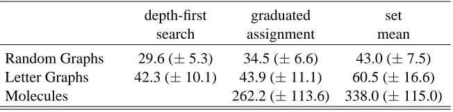
Random Graphs 29.6 (_±5.3) 34.5 (_±6.6) 43.0 (_±7.5) Letter Graphs 42.3 (_±10.1) 43.9 (_±11.1) 60.5 (_±16.6) Molecules 262.2 (_±113.6) 338.0 (_±115.0)

Table 1: Average SSD of sample mean approximated by depth-first search and graduated assign-ment. As reference value the average SSD of the set mean is shown in the last column. Standard deviations are given in parentheses.

each vertex and edge of M0drawn from a uniform distribution over[0,1]d (d=3). Given M0, we

randomly generated k distorted graphs as follows: Each vertex and edge was deleted with 20% probability. A new vertex was inserted with 10% probability and randomly connected to other vertices with 50% probability. Uniform noise from [0,1]d _{with standard deviation σ∈[0,1]was}

imposed to all feature vectors. Finally, the vertices of the distorted graphs were randomly permuted.

We generated 500 samples each consisting of k=10 graphs. For each sample the noise level σ_∈[0,1]was randomly prespecified.

Letter Graphs. The letter graphs were taken from the IAM Graph Database Repository. 5 The graphs represent distorted letter drawings from the Roman alphabet that consist of straight lines only. Lines of a letter are represented by edges and ending points of lines by vertices. Each vertex is labeled with a two-dimensional vector giving the position of its end point relative to a reference co-ordinate system. Edges are labeled with weight 1. We considered the 150 letter graphs representing the capital letter A at a medium distortion level.

We generated 100 samples each consisting or k=10 letter graphs drawn from a uniform distri-bution over the data set of 150 graph letters representing letter A at a medium distortion level.

Chemical Graphs. The chemical compound database was taken from the gSpan site6. The data set contains 340 chemical compounds, 66 atom types, and 4 types of bonds. On average a chemical compound consists of 27 vertices and 28 edges. Atoms are represented by vertices and bonds between atoms by edges. As attributes for atom types and type of bonds, we used a 1-to-k binary encoding, where k=66 for encoding atom types and k=4 for encoding types of bonds.

We generated 100 samples each consisting of k=10 chemical graphs drawn from a uniform distribution over the data set of 340 chemical graphs.

5.1.2 EVALUATIONPROCEDURE

Algorithm 2 (K-Means for Structures)

initialize number k of clusters initialize cluster centers Y1, . . . ,Yk repeat

classify structures Xiaccording to nearest Yj recompute Yj

until some termination criterion is satisfied

5.1.3 RESULTS

Table 1 shows the average SSD and its standard deviation. The results show that using exact sub-gradients gives better approximations of the sample mean than using approximated subsub-gradients. Compared with the set median, the results indicate that the subgradient and approximated subgra-dient method have found reasonable solutions in the sense that the resulting average SSD is lower.

5.2 Central Clustering

Based on the concept of sample mean for structures, we applied the structural versions of k-means and simple competitive learning on four data sets in order to assess and compare the performance of subgradient methods.

5.2.1 CENTRALCLUSTERING ALGORITHMS FORGRAPHS

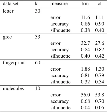
We consider k-means and simple competitive learning in order to minimize the cluster objective (see Section 4.2)7

F(M,

Y

,

X

) =1

2

k

∑

j=1 m

∑

i=1

mi jD(Xi,Yj).

K-means for graphs. The structural version of k-means is outlined in Algorithm 2. This method

operates as the EM algorithm of standard k-means, where the chosen distortion measure in the E-step is D to classify the structures Xiaccording to nearest cluster center Yj. In the M-step the basic

incremental subgradient method described in Algorithm 1 is applied to recompute the means.

Simple competitive learning. The structural version of simple competitive learning corresponds to the basic incremental subgradient method described in Algorithm 1 for minimizing the cluster objective F(X).

5.2.2 DATA

We selected four data sets described in Riesen and Bunke (2008). The data sets are publicly available at the IAM Graph Database Repository. Each data set is divided into a training, validation, and a test set. In all four cases, we considered data from the test set only. The description of the data

5. The repository can be found athttp://www.iam.unibe.ch/fki/databases/iam-graph-database. 6. gSpan can be found athttp://www.xifengyan.net/software/gSpan.htm.