University of New Orleans University of New Orleans
ScholarWorks@UNO
ScholarWorks@UNO
University of New Orleans Theses and
Dissertations Dissertations and Theses
Fall 12-16-2016
Effect of Small-Scale Continental Shelf Bathymetry on Storm
Effect of Small-Scale Continental Shelf Bathymetry on Storm
Surge Generation
Surge Generation
Sunni A. Siqueira
University of New Orleans, [email protected]
Follow this and additional works at: https://scholarworks.uno.edu/td
Part of the Oceanography Commons
Recommended Citation Recommended Citation
Siqueira, Sunni A., "Effect of Small-Scale Continental Shelf Bathymetry on Storm Surge Generation" (2016). University of New Orleans Theses and Dissertations. 2278.
https://scholarworks.uno.edu/td/2278
This Thesis is protected by copyright and/or related rights. It has been brought to you by ScholarWorks@UNO with permission from the rights-holder(s). You are free to use this Thesis in any way that is permitted by the copyright and related rights legislation that applies to your use. For other uses you need to obtain permission from the rights-holder(s) directly, unless additional rights are indicated by a Creative Commons license in the record and/or on the work itself.
Effect of Small-Scale Continental Shelf Bathymetry on Storm Surge Generation
A Thesis
Submitted to the Graduate Faculty of the University of New Orleans in partial fulfillment of the requirements for the degree of
Master of Science in
Applied Physics
by
Sunni Ann Siqueira
B.S. University of New Orleans, 2012
ii
Table of Contents
List of Figures………v
List of Tables………..viii
Abstract……….ix
1. Introduction………1
1.1.Background……….1
1.2.Review of Literature………...2
1.2.1. Storm Parameters……….2
1.2.1.1. Wind Intensity………..2
1.2.1.2. Storm Size………3
1.2.1.3. Translation Speed……….3
1.2.1.4. Landfall Direction………....3
1.2.1.5. Arrival Relative to Tidal Timing……….4
1.2.2. Domain Characteristics………4
1.2.2.1. Domain Size……….5
1.2.2.2. Continental Shelf Slope………...6
1.2.2.3. Continental Shelf Width………..6
1.2.2.4. Perturbations to Local Bathymetry………..6
1.3.Gaps in the Current Knowledge……….7
1.4.Purpose of this Study………..7
2. Methodology………..8
2.1.Overview of Methodology………..8
iii
2.2.1. Design of Regional-Scale Bathymetry……….8
2.2.2. Design of Local-Scale Bathymetry Features………...8
2.2.3. Creation of Local-Scale Bathymetry Features………...11
2.2.3.1. Application of Feature Relief……….11
2.2.3.2. Cross-Shore Depth Selection……….11
2.2.3.3. Alongshore Depth Selection………..13
2.3.Design of Storms………..15
2.3.1. Determination of Storm Parameters………...15
2.3.1.1. Calculation of Maximum Wind Speed………..16
2.3.1.2. Calculation of Central Pressure……….16
2.3.1.3. Calculation of Holland’s B Parameter………...16
2.3.2. Storm Parameters Used in this Study……….16
2.4.Surge Model Description………..17
2.4.1. Simplifying Assumptions (Shallow Water Formulation)………..17
2.4.2. Temporal Discretization……….18
2.4.3. Spatial Discretization……….19
2.4.3.1. Construction of Computational Mesh………19
2.4.4. Implementation of Surge Model………19
2.5.Methods of Analysis……….21
2.5.1. Selection of Recording Station for Elevation Analysis……….21
2.5.2. Calculation of Each Feature’s Influence on Surge Generation………..22
2.5.3. Determination of Feature Influence on Surge Generation by Feature Class…….23
iv
2.5.5. Spatial Analyses to Determine Causes of Observed Surge Response…………...25
3. Results and Discussion………26
3.1.Overview of Results……….26
3.2.Examination of Peak Storm Surge………28
3.2.1. Characteristics of Peak Surge Subject to Differing Storm Conditions…………..28
3.2.2. Effect of Bathymetry Features on Peak Storm Surge………29
3.2.2.1. Overview of Impact of Features on Peak Storm Surge………..29
3.2.2.2. Impact of Bathymetry Features on Peak Elevation………31
3.2.2.3. Impact of Bathymetry Features on Arrival of Peak Surge……….33
3.3.Effect of Bathymetry Features on Surge 3 Hours after Landfall………..38
3.3.1. Surge Response to Shoals by Feature Class………..40
3.3.2. Surge Response to Features Analyzed by Storm Size………...41
3.3.3. Surge Response to Features Analyzed by Storm Track……….41
3.3.4. Surge Response to Features Analyzed by Individual Storm………..42
3.3.4.1. Analysis of Atypical Order of Feature Class Influence……….44
3.4.Effect of Bathymetry Features on Setdown Occurring 4.5 Hour before Landfall during the Small Storm Approaching from the Southeast………...45
4. Conclusion………...48
4.1.Potential Application of Findings……….48
4.2.Future Work………..49
References………52
v
List of Figures
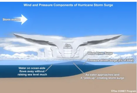
Figure 1-1: Wind and pressure components of hurricane storm surge………1
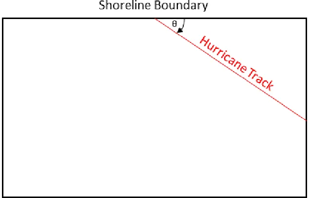
Figure 1-2: Convention for defining storm track angle………...4
Figure 2-1: Plan-view diagram of the 400 by 300 km domain showing feature placement at 25 and 50 km from shore and the location of the continental shelf break 100 km from
shore………...10
Figure 2-2: Cross-shore profiles of the wide features 25 km from shore………..10
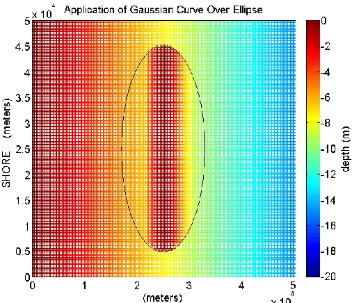
Figure 2-3: Sample sub-domain (plan-view) showing the application of a Gaussian curve over an ellipse, oriented along the major axis, to simulate the relief of a shoal……….11
Figure 2-4: Cross-shore depth selection (shoal)………12
Figure 2-5: Cross-shore depth selection (pit)……….13
Figure 2-6: Sample sub-domain (same as in Fig. 2-3) showing the application of a Gaussian curve over an ellipse, oriented along the major axis, to simulate the relief of a
shoal………...14
Figure 2-7: Depiction of the Cosine-shaped curves (in black) that are part of the alongshore depth selection process used to transition the elevations at the shoal’s ends to the
elevation of the surrounding seafloor………14
Figure 2-8: Final shape of the shoal after alongshore depth selection has been completed……..14
Figure 2-9: The momentum equation with a description of the physical meaning of each
term...18
Figure 2-10: Locations of recording stations in each domain………21
Figure 2-11: Image of the entire domain showing the location of Recording Station 36 relative to the features and the storm tracks………22
Figure 3-1: Elevation in all domains at Recording Station 36 during storms with shore-normal (90°) tracks……….26
Figure 3-2: Elevation in all domains at Recording Station 36 during storms with 60° tracks (approach from the southeast)………27
vi
Figure 3-4: Elevation in all domains at Recording Station 36 during storms with 90° tracks, with inset showing peak elevation in each domain during the smaller (Rm = 42.4 km)
storm………..30
Figure 3-5: Elevation in all domains at Recording Station 36 during storms with 60° tracks, with inset showing peak elevation in each domain during the smaller (Rm = 42.4 km)
storm………..30
Figure 3-6: Elevation in all domains at Recording Station 36 during storms with 120° tracks, with inset showing peak elevation in each domain during the smaller (Rm = 42.4 km) storm………..31
Figure 3-7: Delay in the arrival of surge at Station 36 during the storms approaching from the southeast (60° track)………..33
Figure 3-8: Elevation and water velocity one half hour before landfall in the featureless reference domain (FD) and in the domain with the wide, shallow shoal 25 km from shore (S25W-Sh), during the smaller (42.4 km Rm), more intense storm approaching from the southeast (60° track) ...………..34
Figure 3-9: Elevation and water velocity one half hour before landfall in the featureless reference domain (FD) and in the domain with the wide, shallow shoal 25 km from shore (S25W-Sh), during the larger (60.0 km Rm), less intense storm approaching from the southeast (60° track)………..35
Figure 3-10: Delay in the arrival of surge at Station 36 during the storms (Rm = 42.4 km)
approaching from the southwest (120° track)………36
Figure 3-11: Elevation and water velocity 2.5 hours before landfall in the featureless reference domain (FD) and the domain with the wide, shallow shoal 50 km from shore (S50W-Sh), during the smaller (42.4 km Rm), more intense storm approaching from the southwest (120° track)………37
Figure 3-12: Wind stress 2.5 hours before landfall of the small storm (Rm = 42.4 km)
approaching from the southwest (120° Track)………..37
Figure 3-13: Surge response at Station 36 three hours after landfall in all domains during all six storms……….38
Figure 3-14: Elevation and water velocity 3 hours after landfall in the domains with the wide, shallow shoal at each distance from shore (S25W-Sh and S50W-Sh), during the smaller (42.4 km Rm), more intense storm with a shore-normal approach (90° track)…………..39
vii
Figure 3-16: Examination of feature influence during set-down occurring 4.5 hours before landfall of the small (Rm = 42.4 km) storm approaching from the southeast (60°
track)………..45
Figure 3-17: Wind stress at 4.5 hours before landfall during the storm with a 42.4 km Rm and a 60° tack………..46
Figure 3-18: Elevation and water velocity 4.5 hours before landfall in the domains with the most influential shoal at each distance from shore (S25W-Sh and S50W-Sh), during the
smaller (42.4 km Rm), more intense storm with a 60° track………..46
Figure 4-1: Influence of wide, shallow shoals on surge generation prior to peak surge during the small storm (Rm = 42.4 km) approaching from the southwest (120° track)………...49
Figure 4-2: Influence of the wide, shallow shoals during the setdown that occurred 4.5 hours before landfall during the small storm (Rm = 42.4 km) approaching from the southeast
(60° track)………..50
viii
List of Tables
Table 2-1: Model domains considered in this study with descriptions of their features, if
applicable……….9
Table 2-2: Parameters of the two storms used in this study………..17
Table 2-3 (A-C): Division of the eight shoals into six parameter-based feature classes………...23
Table 2-4 (A-B): Storms grouped by parameter………24
Table 3-1: Maximum elevation (meters) in each domain during each storm at Recording Station 36, colors indicating increase in elevation with decreasing storm size……….28
Table 3-2: Maximum elevation (meters) in each domain during each storm at Recording Station 36, colors indicating increase in elevation with increasing storm track angle…………...29
Table 3-3: Comparison of peak elevation in each domain with a feature to peak elevation in the featureless reference domain (FD)……….32
Table 3-4: Elevation (meters) at Recording Station 36 in each domain three hours after each storm has made landfall……….38
Table 3-5: Comparison of elevation three hours after landfall in each domain with a feature to peak elevation in the featureless reference domain………...39
Table 3-6: Influence of shoal class on surge generation three hours after landfall (mean results for all six storms)………...40
Table 3-7: Influence of shoal class on surge generation three hours after landfall analyzed by storm size………...41
Table 3-8: Influence of shoal class on surge generation three hours after landfall analyzed by storm track………...…..42
Table 3-9: Influence of shoal class on surge generation three hours after landfall analyzed by individual storm……….43
Table 3-10: Influence of shoal class on surge generation four and a half hours before landfall during the storm with a 42.4 km Rm and a 60° track……….47
ix ABSTRACT
Idealized bathymetries were subjected to idealized cyclones in order to measure the storm surge response to a range of bathymetry features, under various storm conditions. Ten
bathymetries were considered, including eight shoals, one pit, and a featureless reference domain. Six storms (two different sizes/intensities and three different landfall directions) were used as meteorological forcing. The bathymetry features influenced local surge response during pre- and post-peak surge conditions. However, peak surge and surge at the coast were not meaningfully affected by the presence of the bathymetry features considered. The effect of three bathymetry feature parameters on surge response was analyzed (i.e. depth below mean sea level, cross-shore width, and distance from shore). Of these parameters, feature depth below mean sea level was the most influential on surge generation.
1
1.
Introduction
1.1.
Background
Simulating oceanographic processes requires specification of ocean depths (bathymetry). Techniques for collecting these data have significantly improved in recent years due to the development of multibeam echo sounders and remote sensing technology, such as LiDAR, allowing for much higher resolution. Increasing resolution of bathymetric data sets necessitates increased storage and data transmission requirements. Additionally, it is more difficult to process and manipulate large data sets than small ones with regard to computer memory requirements. Therefore, it is desirable to reduce the size of the data set through thinning while maintaining fidelity to the surface being represented. The process of thinning removes redundant bathymetric information, which in the case of oceanographic modeling is any bathymetry data that is not necessary to fully represent the processes being modeled. To develop thinning criteria, we must understand the effect of bathymetric features on simulated phenomena. This process begins by considering storm surge generation on the continental shelf.
2
Storm surge is a change in sea level accompanying a hurricane or other intense storm, whose height is the difference between the sea surface's observed level and the level that would have occurred in the absence of the storm. During a hurricane, storm surge is produced by water being pushed toward the shore by the force of the winds moving cyclonically around the area of low pressure located at the center of the storm (Figure 1-1). Friction between the wind and the water allows the water to be pushed in the direction of the wind's motion. The low pressure of the storm system contributes to increased sea surface elevation, this is known as the inverted barometer effect; however, the impact on surge of the low pressure is minimal in comparison to the water being forced toward the shore by the wind. Tides and surface waves also contribute to the sea surface elevation and can magnify surge elevations, but their effects are not included in this study.
The geometry of the continental shelf is another important factor influencing storm surge. In shallow water the slope the water surface must take to balance the force of the cross-shelf winds is inversely proportional to the depth of the water (Pugh, 1996). This relationship is due to the fact that the force of the winds is acting on a smaller volume of water in a shallow area than in an equal area of deep water. Wide, shallow shelves experience greater storm surge than narrow or steeply sloping shelves under the same storm conditions. Wide shelves experience greater surge because there is a larger distance over which surge can be generated, and since surge is inversely proportional to water depth (and to bottom slope), shallow shelves generate more surge than deep or steeply sloping shelves. Since the generation of surge is sensitive to water depth, the geometry of smaller scale features on the continental shelf, such as shoals and pits may, also influence surge. It is the goal of this study to determine such features' influence on storm surge generation.
1.2.
Review of Literature
Considerable research has been undertaken to understand various influences on the generation of storm surge in the coastal zone (Blain et al., 1994; Irish et al., 2008; Rego and Li, 2009; Weaver and Slinn, 2010; and Li et al., 2013). To date, these influences can be divided into two categories: 1) storm parameters such as wind intensity, storm size, translation speed, landfall direction, and arrival relative to tidal phase, and 2) physical characteristics of the environment, for example, continental shelf slope, width, and features. The following sections summarize the current understanding of how these various parameters affect the generation of storm surge in coastal waters.
1.2.1.
Storm Parameters
Hurricanes are characterized by several defining characteristics, their intensity measured as wind speed, their size as a function of the radius to the band of winds having maximum speed (Rm), and their translation speed. Surge generation is also affected by the direction of the storm’s
approach to land, as well as its arrival relative to the tidal phase. The breakdown of each hurricane parameter and its influence on surge generation is presented.
1.2.1.1. Wind Intensity
3
predictor of the wind damage expected by a hurricane, it alone is not the best predictor of storm surge. This is particularly true in the case of intense storms on mildly sloping continental shelves because surge generation is proportional to the square of the wind velocity as well as inversely proportional to the bottom slope.Rego and Li (2009) found that increasing wind intensity results in the increase of both flooded volumes and peak surge elevation. They also discovered that wind intensity has a more significant impact on peak surges as compared to the Rm. While testing the
sensitivity of peak surge to domain size under differing storm intensities, Li et al. (2013) showed that with other parameters fixed, an increase in storm intensity causes an increase in peak surge.
1.2.1.2. Storm Size
Irish et al. (2008), Rego and Li (2009), and Li et al. (2013) also considered the influence of storm size on surge generation. Irish et al. (2008) found that for a given storm intensity, peak surge increases with increasing Rm. This relationship holds for all bottom slopes. Their numerical
results indicate that the role of storm size in surge generation becomes much more important on mildly sloping bottoms and for intense storms. Surge generation is inversely proportional to bottom slope and proportional to wind stress, and a larger storm increases the fetch and duration over which winds can act.Historical observations were also used to support these findings. Rego and Li (2009) found that similar to increasing wind intensity, increasing a storm’s Rm results in
the increase of both flooded volumes and peak surge elevation. In keeping with the results of Irish et al. (2008), Li et al. (2013) found that peak surge increases with increasing Rm.
1.2.1.3. Translation Speed
Irish et al. (2008), Rego and Li (2009), and Li et al. (2013) investigated the influence of hurricane translation speed on peak surge. The results of Irish et al. (2008) indicate a correlation between storm translation speed (values from 2.6 to 10.2 m s-1) and peak storm surge for steep to moderate bottom slopes. When the bottom slope is≤ 1:2500, a 50% increase in forward speed translates to a 15%–20% increase in peak surge. Of the cases they investigated, only the case with the mildest bottom slope (1:10,000) did not experience an increase in peak elevation with increased translation speed. Rego and Li (2009) found that a hurricane’s forward speed has significant positive effect on peak surge heights but a significant negative effect on total
maximum flooded volumes. For example, a slower storm produces lower peak surges that travel far inland, whereas a faster hurricane will move rapidly across the shoreline generating higher surges but flooding a relatively narrower section of the coast. Li et al. (2013) found that peak surge increases with increasing hurricane translation speed for speeds less than 12 m s-1, and it remains the same for forward speeds between 12 and 21 m s-1.
1.2.1.4. Landfall Direction
4
Figure 1-2: Convention for defining storm track angle. Storm tracks are described using positive angles in which θ is the angle rotating from the right side of the shoreline to the hurricane track in a clockwise direction.
Irish et al. found that all storm tracks with more westerly headings (45°-75°) produced smaller surges than the due north (90°) track for both moderately and mildly sloping bottoms. For the most mildly sloping bottom (1:10,000), storms with more easterly headings (105°-150°) produced surges that were as large, or slightly larger (no more than 8%), than the due north (90°) track. These results were for storms with a forward speed of 5.1 m s-1. Li et al. conclude that landfall direction could affect simulated surge level dramatically, having a greater impact than
Rm and translation speed. They tested twelve different storm tracks and found that peak surge
was highest when a hurricane makes landfall with a 90° track (bottom slope 1:1,500).
1.2.1.5. Arrival Relative to Tidal Timing
As one might expect, Rego and Li (2009) confirmed that hurricanes landfalling at high tide yield both greater flooded volumes and peak surges than those landfalling at low tide. They considered the cases of double amplitude and normal amplitude tides with the storm landfalling at high and low tide for each of the tidal amplitudes. Variations are only about ±16% of the inundation volume of the simulation without tidal forcing. They also found that tide-surge nonlinearity decreases the impact of high- or low-tide landfalls. For example, peak storm tides for high tide and double high tide should be greater than the no tide case by about 0.33 and 0.66 m (the tidal amplitude), and they are not.
1.2.2.
Domain Characteristics
5 1.2.2.1. Domain Size
Blain et al. (1994) compared hurricane storm surge generation in three domains of differing sizes, subject to two different open boundary forcings, in order to determine the influence of domain size on storm surge response. All of the domains had identical bathymetry and identical discretization in the areas they held in common. Much of the small (Florida coast) domain was on the continental shelf at depths of < 130 m, and its boundaries were almost exclusively across the continental shelf. The medium (Gulf of Mexico) domain contained the small domain and all surrounding regions in the Gulf of Mexico. It had two open ocean boundaries; one across the Strait of Florida and one across the Yucatan Channel. The large (Eastcoast) domain contained the medium domain and also included the western North Atlantic Ocean and the Caribbean Sea. Its open ocean boundary was the entire stretch of ocean along the 60° W meridian from Nova Scotia in the North to Venezuela in the South.
The small domain underestimated surge using both boundary condition specifications considered in the study and cannot be used to obtain a physically relevant storm surge response. This is because an appropriate elevation boundary condition cannot be specified at the cross-shelf boundaries because in order to do so, the storm surge generated on the cross-shelf would need to be known in advance. The domain was also too small relative to the spatial scale of a hurricane. In the medium domain, the two open ocean boundaries significantly influenced the setup of modes in the Gulf of Mexico. The frequency of the modes varied with the application of
different boundary conditions (i.e., it was highly sensitive to boundary condition specification), and this domain had shortcomings in the representation of basin to basin dynamics. The large domain was insensitive to boundary condition specification. Simulations using this domain give good results even without the elevation boundary condition being precisely known. It was much better at representing basin to basin dynamics, as evidenced by the more natural resonant modes in the Gulf of Mexico. In order to obtain the most realistic results, it is best for the open
boundary to be far from the intricate processes that occur on the continental shelf and the within the basin in response to the hurricane.
Li et al. (2013) also show that simulated storm surge is significantly affected by domain size especially when the modeled domain is relatively small. In keeping with Blain et al. (1994), they found that peak surge is underestimated when the model domain used is too small.
However, when the domain size is greater than a given threshold, they found that simulated storm surge is insensitive to domain size. One difference between the two studies is that Li et al. (2013) used rectangular idealized domains free from basin to basin interaction. Li et al. (2013) determined the threshold domain size for ranges of wind intensities, Rm, translation speeds,
landfall directions, bottom slopes, and continental shelf widths. Their results indicate that this threshold domain size is not sensitive to storm intensity but increases linearly with increasing hurricane Rm. When a hurricane approaches land perpendicularly, the threshold domain size
6 1.2.2.2. Continental Shelf Slope
Irish et al. (2008), Weaver and Slinn (2010), and Li et al. (2013) consider the influence of continental shelf slope on storm surge generation. Irish et al. found that for a given storm,
decreasing bottom slope results in increased peak surge. Relating to storm size, their parameter of interest, they discovered that the linear trend of increasing peak surge with increasing storm size becomes steeper as shelf slope becomes milder, implying that the role of storm size in producing surge becomes increasingly important over mildly sloping bottoms. When examining the combined influence of forward speed and bottom slope on surge generation, with the
exception of their most mildly sloping bottom (1:10,000), increasing forward speed resulted in increasing surge with decreasing slope. Weaver and Slinn examined behavior of storm surge on slopes ranging from 1:20 to 1:200 in their 1D simulations. In these cases, the slopes extended 50 km offshore. To develop their baseline data set they generated surge predictions on the sloped profiles in the absence of any bathymetric perturbations. With all other factors held constant, they found that peak surge was inversely proportional to shelf slope. Li et al.’s results show that peak surge increases with decreasing bottom slope which corresponds to Irish et al.’s and Weaver and Slinn’s findings. Additionally, they found that the required domain size decreases with increasing bottom slope.
1.2.2.3. Continental Shelf Width
Li et al. (2013) discovered that peak surge increases with increasing shelf width for shelves less than 100 km and is not sensitive to increases in shelf width beyond 100 km.
1.2.2.4. Perturbations to Local Bathymetry
Weaver and Slinn (2010) examined the extent to which variations in nearshore
bathymetry affect the storm surge at the coast. They created a 1D idealized bathymetry which was altered by adding a local Gaussian disturbance at various distances from the shoreline. For each of the bottom slopes considered a suite of Gaussian disturbances was created. The
perturbations were defined by their amplitudes (percentage of the local water depth), their widths (100 to 5000 m), and the distance from shore to their centers (500 to 5000 m). They found that storm surge at the coast varied only slightly as a consequence of local variation in the
bathymetry, with the bulk of the simulations predicting the surge levels at the shore to be very close to that of the unperturbed bottom.
They found that the resulting surge varied by ±10% for amplitude variations that were less than ±40% of the initial bathymetry. Fluctuations up to +60% would generate a difference at the coast of at most +20%. As the perturbations’ amplitudes become larger, they found that the cases of extreme width and proximity to the shoreline start to produce outliers in the results. Depending on the maximum acceptable root-mean-square deviation (RMSD) allowed, one can allow for a large range of bathymetric variations without significantly changing the surge results at the shoreline.
Weaver and Slinn (2010) also looked at the relative surge versus the width of the perturbation, finding that the wider disturbances generated a greater deviation from the
7
bathymetric fluctuations at the shore begin to diminish. They note that for all cases this limit coincides with a depth of about 30 m, and they call this the depth of relative influence (DRI). Seaward of that limit, the effects of altering the bathymetry on surge begin to diminish.
Two-dimensional simulations conducted by Weaver and Slinn (2010), in which they perturbed the bathymetry in locations affected by the historical storms used as forcing for those simulations, led to results that were consistent with their 1D findings.
1.3.
Gaps in the Current Knowledge
Most of the recent studies considered (Irish et al., 2008; Weaver and Slinn, 2010; Li et al., 2013) considered factors affecting only peak surge generation or peak surge and inundation (Rego and Li, 2009). The study presented herein will address the complete time evolution of surge, with a focus on surge recession. With the exception of Weaver and Slinn, past focus has been on surge generation at the shoreline by considering surge generation offshore. In our study the focus is between 5 km and 70 km offshore. While Weaver and Slinn did examine the
influence of bathymetric perturbations on surge generation, they only consider their influence on peak surge. In their 1-D simulations Weaver and Slinn made qualitative remarks about the influence of a bathymetric perturbation's cross-shore width and distance from shore on peak surge, quantifying only the influence of amplitude. The study herein extends this work by
quantifying the influence of feature parameters (i.e., amplitude, cross-shore width, distance from shore) on the generation of storm surge. In the 2-D studies of Weaver and Slinn, perturbations to the local bathymetry are much smaller in area than the features considered in this study and have only ± 20% change in elevation to the surrounding bathymetry. The features considered in this study are larger, farther from shore, and on a more gently sloping continental shelf than the bathymetric perturbations that they used in their 2-D simulations. In their 2-D simulations, Weaver and Slinn do examine the perturbations’ influence on local influence surge, not just at the shoreline, but only at peak elevation.
1.4.
Purpose of this Study
8
2.
Methodology
2.1.
Overview of Methodology
To determine the influence of offshore bathymetric features on storm surge, numerical simulations utilizing idealized domains and tropical cyclones were conducted. Additionally, the sensitivity of surge to storm landfall direction and to storm size was considered, both in the presence and absence of the bathymetric features. The next sections describe the design of the domains, including their features, the design of the storms, and provide a description of the storm surge simulator, ADCIRC. The analysis techniques are also discussed in detail.
2.2.
Domain Design
2.2.1.
Design of Regional-Scale Bathymetry
Each domain represents ocean depths from the shoreline, over the continental shelf and slope, and out into the deep ocean through the application of idealized geometries for each of the geomorphic components, the shoreline, continental shelf, continental slope, and the abyssal plain. Each domain is rectangular, with dimensions of 400 km alongshore and 300 km cross-shore. These dimensions exceed the threshold domain size needed to prevent underestimation of surge, as defined in Li et al. (2013), for the chosen continental shelf characteristics and storm parameters, as described below. Depth contours are shore-parallel (Irish et al., 2008; Li et al., 2013), and each region (i.e. shelf, slope, abyssal plain) has a constant slope. The continental shelf width is 100 km, which is the width at which peak surge becomes insensitive to increasing shelf width according to Li et al. (2013). Its slope is 0.0003, which is representative of the gently sloping shelves off the coasts of Louisiana (Irish et al., 2008). Depths over the shelf range from 0 to 30 m, which means that the entire continental shelf lies within the range of the depth of
relative influence (DRI) defined by Weaver and Slinn (2010). The slope of the continental slope section is 0.04, which is the global average (Wefer, 2003), and its depths range from 30 to 2000 m. The depth of the abyssal plain for this application is set to 2000 m. The reference domain has no bathymetric feature on its continental shelf (featureless) and is of uniform depth in the
alongshore dimension. Other domains are identical to the reference domain except at the location of their features.
2.2.2.
Design of Local-Scale Bathymetry Features
Just as the large-scale geomorphic components were represented using idealized
geometries, the bathymetry features on the continental shelf were also simulated using idealized geometries. The relief in the cross-shore direction was modeled using a Gaussian curve over an ellipse, and the alongshore edges were then smoothed using cosine-shaped curves. Three
9
feature is subaerial. A domain containing a depressed feature (pit) and a featureless reference domain were also constructed.
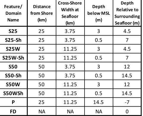
For this study, all features were 50 km long in the alongshore direction and located in the center of the domain with respect to the alongshore direction. Each shoal was defined by three parameters, 1) its distance from shore, either 25 or 50 km; 2) its cross-shore width, either 3.75 or 11.25 km; and 3) its depth relative to mean sea level (MSL), either 0.5 or 3 m below MSL. The combination of these parameters resulted in 8 unique raised features. A single depressed feature (pit) was considered. It had the dimensions and location of the most influential raised feature but an inverse amplitude (7 m below the surrounding seafloor rather than protruding 7 m above the surrounding seafloor).
Table 2-1 lists each domain considered in this study and provides a detailed description of their features, where applicable. With the exception of the reference domain, which has no bathymetry feature on its continental shelf, domains were named for their features. The domain name convention that is used throughout this document it as follows: FD is the featureless
reference domain, S indicates shoal, P indicates pit; 25 or 50 indicates feature distance (km) from shore; W indicates the wider, 11.25 km features; and -Sh indicates the shallower features that are 0.5 m below mean sea level (MSL). For example, S50W-Sh, indicates the domain has a shoal 50 km from shore with the wider (11.25 km) width and the shallower (0.5 m) depth below MSL. A second example, S25, indicates the domain has a shoal centered 25 km from shore with the narrower (3.75 km) width and the deeper (3.0 m) depth below MSL.
Table 2-1: Model domains considered in this study with descriptions of their features, if applicable.
Figure 2-1 depicts the 400 by 300 km domain in plan-view, showing the locations and widths of the features chosen for this study. The location of the continental shelf break is also shown. The alternative values of two of the parameters that were varied (feature distance from shore and cross-shore width) are clearly visible in Figure 2-1. The alternative values of feature depth below MSL are shown in Figure 2-2.
Feature/ Domain Name Distance from Shore (km) Cross-Shore Width at Seafloor (km) Depth below MSL (m) Depth Relative to Surrounding Seafloor (m)
S25 25 3.75 3 4.5
S25-Sh 25 3.75 0.5 7
S25W 25 11.25 3 4.5
S25W-Sh 25 11.25 0.5 7
S50 50 3.75 3 12
S50-Sh 50 3.75 0.5 14.5
S50W 50 11.25 3 12
S50WSh 50 11.25 0.5 14.5
P 25 11.25 14.5 -7
10
Figure 2-1: Plan-view diagram of the 400 by 300 km domain showing feature placement at 25 and 50 km from shore and the location of the continental shelf break 100 km from shore. The two possible feature widths are shown at each location.
11
2.2.3.
Creation of Local-Scale Bathymetry Features
2.2.3.1. Application of Feature Relief
The process of creating realistic features using idealized geometries is outlined below. In plan-view each bathymetry feature is elliptical in shape. To create a feature’s elevation, depths associated with a Gaussian function are applied over the ellipse. The surface formed is
symmetric with respect to the major axis of the ellipse, which runs in the alongshore direction.
Figure 2-3: Sample sub-domain (plan-view) showing the application of a Gaussian curve over an ellipse, oriented along the major axis, to simulate the relief of a shoal. In this image, cross-shore depth selection has already been performed, but alongshore depth selection has not.
2.2.3.2. Cross-Shore Depth Selection
12
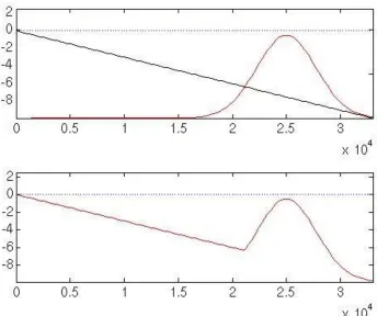
Figure 2-4: Cross-shore depth selection (shoal): (Top) The blue dotted line represents the water’s surface. The black line represents the cross-shore profile of the continental shelf in the absence of a feature, and the red curve
represents the Gaussian curve used to create the cross-shore profile of the shoal. The depths of the two shapes are compared at each point along the x-axis (cross-shore), and from the shore to the offshore side of the feature, the shallower depth is retained as the depth of the seafloor at that location. Beyond the offshore side of the feature (not pictured), the deeper of the two depths is the one retained, which is the elevation of the continental shelf. (Bottom) The blue dotted line represents the water’s surface, and the red curve shows the cross-shore profile after the depth selection process has been completed.
13
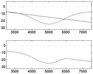
Figure 2-5: Cross-shore depth selection (pit): (Top) The blue dotted line represents the water’s surface. The black line represents the cross-shore profile of the continental shelf in the absence of a feature, and the red curve
represents the inverted Gaussian curve used to create the cross-shore profile of the pit. The depths of the two shapes are compared at each point along the x-axis (cross-shore), and from the shore to the nearshore side of the feature (not pictured), the shallower depth is the one retained, which is the depth of the continental shelf. From the
nearshore side of the feature through the most offshore extent of the continental shelf, the deeper elevation is the one retained. (Bottom) The blue dotted line represents the water’s surface, and the red curve shows the cross-shore profile after the depth selection process has been completed.
2.2.3.3. Alongshore Depth Selection
At the ends of the features, depth changes abruptly when going from the Gaussian depths applied over the ellipse to the depths of the surrounding seafloor (Figure 2-6). In order to avoid unrealistic discontinuities in the bathymetry, smoothing of the ends of the features is
14
Figure 2-6: Sample sub-domain (same as in Fig. 2-3) showing the application of a Gaussian curve over an ellipse, oriented along the major axis, to simulate the relief of a shoal. In this image, cross-shore depth selection has already been performed, but alongshore depth selection has not.
Figure 2-7: Depiction of the cosine-shaped curves (in black) that are part of the alongshore depth selection process used to transition the elevations at the shoal’s ends to the elevation of the surrounding seafloor. The alongshore depth selection process involves comparing the elevation of the cosine-shaped curve and the elevation of the feature at each point along the y-axis (alongshore). For shoals, the deeper of the two elevations is retained at each point of comparison.
15
2.3.
Design of Storms
The tropical cyclones used as forcing for the storm surge model are captured by a
simplistic but canonical analytic model by G. J. Holland, Holland (1980). Analytic models arose from the need to recreate storms based on sparse observations. The Holland model is based on the cyclostrophic approximation for wind speed, Vc:
𝑉𝑐 = [𝐴𝐵(𝑝𝑛− 𝑝𝑐) exp (−𝐴
𝑟𝐵) /𝜌𝑟
𝐵], (2-1)
where A and B are scaling parameters, pn is the ambient pressure, pc is the central pressure, r is
the radius, and ρ is the air density (assumed to be constant at 1.15 kg/m3). The radius to maximum winds is Rm = A1/B, so A can be expressed as RmB.
In order to create sea level pressure and wind profiles, the Holland model requires the input of the following parameters (Eq. 2-1): radius of maximum winds (Rm) used to determine A,
Holland's B parameter (B), central pressure of the storm (pc), and environmental (ambient)
pressure (pn). The determination of these parameters will be discussed in detail in Section 2.3.1.
Radius of maximum winds is the distance from the center of a tropical cyclone to the location of the cyclone's maximum winds. In well-developed hurricanes, the radius of maximum winds is generally found at the inner edge of the eyewall (Clements, 2009). Theshape of the pressure profile is controlled by Holland’s B parameter. Holding the radius of maximum winds constant, increasing B causes expansion of the eye and concentrates the pressure drop near the radius of maximum winds, resulting in a steeper gradient. Lower B values cause a more gradual pressure drop beginning near the center of the storm. Larger B values adjust the wind field to give stronger winds near the radius of maximum winds and weaker winds at larger radii (Holland, 1980). Central pressure of the storm and environmental pressure are used to calculate a pressure difference. The value used for environmental pressure is the standard atmospheric pressure of 1013.25 hPa.
Additionally, the storm’s track and forward speed are needed by the Holland model in order to generate the time varying wind and pressure fields. The storm’s track describes the path that the eye of the storm takes, and forward speed is the translation speed of the storm system (in contrast to rotational speed of the system or maximum velocity, Vm, of the winds). The storm’s
track and forward speed are incorporated into the Holland model via the longitude and latitude coordinates of the storm’s center at 15 minute intervals. All storms used in this study have a uniform forward speed of 6.0 m/s.Three track orientations are used this study: 60, 90, and 120 degrees relative to the landfalling shoreline boundary. (Refer to Figure 1-2 for the definition of track angle.) The spatial resolution of the storm data produced by the hurricane model is 250 m. This value was chosen because 250 m is the highest resolution of the computational mesh used in the surge model.
2.3.1.
Determination of Storm Parameters
Two storm sizes were chosen for this study, Rm = 42.4 km and Rm = 60.0 km, in order to
16
generally more intense than larger storms so, typically, as Rm decreases, storm intensity
increases. Given that storm size was prescribed, realistic values for other required parameters were calculated using the following relationships.
2.3.1.1. Calculation of Maximum Wind Speed
The maximum wind speed, Vm, for each size storm was found using Eq. 2 from Gross et
al. (2004). The latitude, θ, chosen is 30° N because locations at this latitude are commonly affected by tropical cyclones, and it is appropriate to the Northern Gulf of Mexico.
𝑅𝑚 = 35.37 − 0.111𝑉𝑚+ 0.570(𝜃 − 25), (2-2)
where 𝑅𝑚 = radius of maximum winds (nmi)
𝑉𝑚 = maximum wind (kt)
𝜃 = latitude (ºN)
2.3.1.2. Calculation of Central Pressure
Knaff and Zehr (2007) fit a wind-pressure relationship (WPR) based on gradient wind balance to the dataset used by Atkinson and Holliday (1975) that Knaff and Zehr binned by storm intensity. Given the maximum wind speed, Vm, and a reference pressure, Pref, the central
pressure is obtained from a table provided by Knaff and Zehr (2007) that is based on the equation:
∆𝑝 = 11.48 − 0.73𝑉𝑚− ( 𝑉𝑚
107.21) 2
, (2-3)
where ∆𝑝 = 𝑃𝑟𝑒𝑓− 𝑝𝑐
𝑝𝑐 = central pressure (hPa)
𝑃𝑟𝑒𝑓 = 1010 (hPa), the value for Penvused by Knaff and Zehr (2007) 𝑉𝑚 = maximum wind (kt)
2.3.1.3. Calculation of Holland’s B Parameter
Using the values for the storm’s central pressure, pc, environmental pressure, pn, and the
radius of maximum winds, Rm, Holland’s B parameter can be calculated using Eq. 5 from
Vickery and Wadhera (2008):
𝐵 = 1.38 − 0.00184∆𝑝 + 0.00309𝑅𝑚, (2-4)
where 𝐵 = Holland’s B parameter
∆𝑝 = the difference between the environmental pressure 𝑝𝑛 and central pressure 𝑝𝑐 (hPa)
𝑅𝑚 = radius of maximum winds (km)
2.3.2.
Storm Parameters Used in this Study
The values of the parameters used in creating each storm can be found in Table 2-2. The maximum wind speeds of the storms with a Rm of 60.0 km correspond to a tropical storm
(Webster et al., 2005). The storms with a Rm of 42.4 km have maximum wind speeds and central
17
Table 2-2: Parameters of the two storms used in this study. The smaller, more powerful storm’s parameters are in pink, and the larger, more diffuse storm’s parameters are in lavender.
2.4.
Surge Model Description
The ADvanced CIRCulation (ADCIRC) model is a highly developed computer program for solving the equations of motion for a moving fluid on a rotating earth (Luettich et al., 1992). ADCIRC was developed to provide a more accurate technique for predicting sea surface
elevation and currents in coastal areas. It is used for computing features of circulation patterns driven by tides, wind, and atmospheric pressure gradients (Luettich et al., 1992), and it is widely used for modeling storm surge (Blain et al., 1994; Irish et al., 2008; Rego and Li, 2009; Weaver and Slinn, 2010; and Li et al., 2013) and coastal inundation (Rego and Li, 2009). ADCIRC utilizes highly flexible unstructured grids based on finite elements. This allows for excellent characterization of complex geometries with the ability to have high resolution in areas of interest and lower resolution away from those areas. Therefore, one can have a large domain allowing for the use of open water boundary conditions without having to include large quantities of information to characterize areas far from the region of interest (Luettich et al., 1992).
2.4.1.
Simplifying Assumptions (Shallow Water Formulation)
ADCIRC is designed to model long-wave circulation by applying the Reynolds-averaged, Navier-Stokes equations, simplified using the Boussinesq and the hydrostatic pressure
approximations. As a result, ADCIRC’s solutions are valid for nearly horizontal flow. Inherent in this formulation are the following assumptions (Kinnmark, 1985):
1. Reynolds-averaging – An approximate time-averaged solution for velocity can be obtained through separating flow into mean and fluctuating quantities and treating the fluctuating part of the solution (turbulence) using vertical turbulent closure.
2. Boussinesq approximation – Density fluctuations are small, and in terms where density is not multiplied by gravitational acceleration, the variation in density can be replaced by a constant value for density.
3. Hydrostatic approximation – Vertical accelerations are small compared to the
acceleration of gravity (the horizontal scale is far greater than the vertical scale so that there is negligible variation in density over the depth) so that the vertical pressure gradient may be given as the product of density, gravity, and depth.
Radius to Maximum Winds (km) Holland's B Parameter Central Pressure (hPa) Maximum Wind Speed (m/s) Forward Speed (m/s)
42.4 1.34 919 71.0 6.0
60.0 1.51 983 27.0 6.0
18
ADCIRC Two-Dimensional Depth-Integrated (2DDI) solves the Generalized Wave Continuity Equation (GWCE) (Equation 2-5), which is a linear combination of the depth-integrated primitive continuity equation (PCE) (Equation 2-6) and the depth-integrated momentum equation (M) (Equation 2-7).
𝜕(𝑃𝐶𝐸)
𝜕𝑡 + 𝜏0(𝑃𝐶𝐸) − 𝛻 ∙ 𝑀 = 0 (2-5)
τ0 is the GWCE weighting parameter used to optimize numerical accuracy, where τ0 → ∞ results
in a pure wave equation and τ0 → 0 results in a pure continuity equation. The GWCE formulation
prevents the generation of non-physical solutions that can arise from finite element (FE)
discretization of the PCE. It also allows for time-independent system matrices which require less computational resources than time-dependent matrices that must be assembled and solved at every time step. The GWCE formulation is applied prior to any numerical discretization (Kinnmark, 1985).
𝜕𝜁 𝜕𝑡+
𝜕𝑈𝐻 𝜕𝑥 +
𝜕𝑉𝐻
𝜕𝑦 = 0, (2-6)
where ζ = free surface elevation relative to the geoid
H = ζ + h is the total water depth to the free surface, where h = bathymetric depth relative to the geoid
U = zonal depth-averaged horizontal velocity
V = meridional depth-averaged velocity
𝜕𝐯
𝜕𝑡+ 𝐯𝛻 ∙ (𝐯) + 𝐟 × 𝐯 + 𝛻 [ 𝑝𝑎
𝜌0+ 𝑔(𝜁 − 𝛼𝜂)] −
𝝉𝑠+𝝉𝑏
𝜌0𝐻 −
𝜺 𝐻𝛻
2(𝐻𝐯) = 0 (2-7)
For the momentum equation (Equation 2-7), the physical meanings of the terms are described in Figure 2-9.
Figure 2-9: The momentum equation with a description of the physical meaning of each term.
2.4.2.
Temporal Discretization
19
solution at the previous time step. Explicit methods are computationally inexpensive to implement, but they can suffer from instabilities if the Courant–Friedrichs–Lewy (CFL) condition is not met. This criterion is a ratio of the time step to the spatial interval (or some power of the spatial interval based on the order of the differential equation being approximated) and thus restricts how large a time step can be used in order to not have, e.g., a wave travel a greater distance than the highest mesh resolution in one time step, resulting in inaccuracies (Courant et al., 1967). ADCIRC uses different temporal discretization for the continuity and momentum equations. For the continuity equation, the time derivatives are discretized over three levels, so that the solution for the future water level requires knowledge of the present and past water levels. For the momentum equation, the temporal discretization is explicit for all terms except Coriolis, which uses an average of the present and future velocities (Luettich et al., 1992).
2.4.3.
Spatial Discretization
Finite element (FE) discretization is applied to the time-discretized form of the governing equations to complete their conversion into systems of algebraic equations suitable for numerical solution. The FE method is a numerical technique used to approximate the solution to a
boundary-value problem, which is a differential equation together with a set of boundary conditions. The FE technique uses variational methods to minimize an error function and produce a stable solution. ADCIRC uses a continuous Galerkin FE method. The FE method provides maximum grid flexibility and allows highly efficient numerical solutions to be obtained using model domains that include complicated bathymetries and shoreline geometries that also stretch considerable distances offshore to implement open-water boundary conditions (Luettich et al., 1992). FE algorithms based on triangular elements are highly flexible and can provide local grid refinement in a systematic and optimal fashion (Luettich et al., 1992). The ability to vary resolution over the domain (grid flexibility) is pivotal to solution accuracy and
computational efficiency. Accuracy is improved by having high resolution near shore and in areas where flow and/or geometry vary rapidly. The ability to have lower resolution away from areas of high variation reduces the computational resource requirement.
2.4.3.1. Construction of Computational Mesh
Creation of the computational meshes was accomplished using xmGredit5 (Turner, 1999) and MeshGUI (Blain et al., 2008). The finite element mesh of each domain, consisting of
triangular elements, had 4,000 m resolution over the abyssal plain. Four depth-based refinements were made at depths of 1,990 m, 1,340 m, 690 m, and 40 m, resulting in 250 m resolution just before reaching the continental shelf break, and continuing to shore. The featureless reference domain had 796,743 nodes and 1,590,625 elements.
2.4.4.
Implementation of Surge Model
Simulations are performed using ADCIRC v50.99.05 in barotropic, two-dimensional depth-integrated mode (2DDI). Two boundary types are used, an elevation boundary at the open water edges of the domain and a mainland boundary at the shore. Elevation, η, was specified at each node of the open water boundary. It was chosen to be constant and equal to MSL (η = 0.0000). The shore boundary allowed no normal flow but had no constraint on tangential flow, as it was
representative of a mainland boundary. Wind stress and atmospheric pressure were input to all grid nodes every 15 minutes (900 s), which is not equal to the model time step (1 s), so
20
time step. Wetting and drying of elements was enabled, and the depth for a node and surrounding elements to be considered dry was 0.01 m. A dry node wets if a water surface slope exists that would drive water from a currently wet node to the dry node and the steady-state current velocity that results would have a velocity > 0.01 ms-1. Initial water depths were assumed equal to the bathymetric water depth specified in the grid file. A hybrid nonlinear bottom friction formulation was used (Equation 2-8).
𝐶𝐷 = 𝑚𝑎𝑥 {𝐶𝐷 𝑚𝑖𝑛(1 + (𝐻𝑏𝑟𝑒𝑎𝑘
𝐻 ) 𝜃
)
𝛾 𝜃
, 10−4}, (2-8)
where CD min is either a linear or quadratic drag coefficient, H is the total water column depth,
and Hbreak is the depth at which waves break. According to Luettich and Westerink (1995), the
exponent θ determines how rapidly CD approaches each asymptotic limit, while the exponent γ
21
2.5.
Methods of Analysis
2.5.1.
Selection of Recording Station for Elevation Analysis
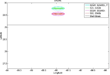
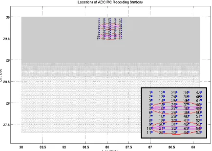
Figure 2-10: Locations of recording stations in each domain. Elevation and velocity were recorded at 15 minute intervals throughout the simulations at these locations (global elevation and velocity were recorded hourly). An enlarged view of the stations, shown with respect to the features’ locations, is shown in the lower right corner of the figure.
22
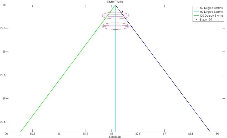
Figure 2-11: Image of the entire domain showing the location of Recording Station 36 relative to the features and the storm tracks. Station 36 is in a location where the northeast quadrant of each storm passes over. Though the tracks appear to end at the shore (top of the image), the storms progress inland beyond the shoreline allowing the storm conditions over water to gradually diminish.
After completion of the simulations, elevations at Recording Station 36 in all ten domains were compared for each storm, looking for differences in elevation between the domains. Times at which to examine the surge response were chosen based on the occurrence of elevation differences, indicating feature influence on surge response at that time. Even though there was not a noticeable difference in elevation in the various domains at the time of maximum elevation, peak surge was still considered to be of interest. The other times at which surge response to the features was examined were three hours after landfall for all storms and four and a half hours before landfall during a particular storm in which there was a large difference in elevation from one domain to the next.
Once the times at which the features influenced surge were determined, the following techniques were employed to determine which feature characteristics were most influential to surge generation and how the surge response varied under different storm conditions.
2.5.2.
Calculation of Each Feature’s Influence on Surge Generation
At each time of interest (i.e. peak surge, three hours after landfall, and during the pre-landfall set-down that occurred during one storm), the difference in elevation (cm) between domains with features and the featureless reference domain (FD) was calculated:
𝐸𝑙𝑒𝑣𝑎𝑡𝑖𝑜𝑛 𝐷𝑖𝑓𝑓𝑒𝑟𝑒𝑛𝑐𝑒 (𝑐𝑚) = (𝜂𝑖 − 𝜂0) × 100, 𝑖 ≠ 0, (2-9)
where η0 is the elevation in the featureless reference domain (FD), and ηi represents elevation in
23
Secondly, elevations in domains with features were compared with the elevation in the FD to determine percent change in elevation from the FD:
% 𝐶ℎ𝑎𝑛𝑔𝑒 𝑓𝑟𝑜𝑚 𝐹𝐷 =𝜂𝑖−𝜂0
|𝜂0| × 100 , 𝑖 ≠ 0, (2-10)
where η0 is the elevation in the featureless reference domain (FD), and ηi represents elevation in
a domain with a feature.
Elevation difference in centimeters from the FD and percent change from the FD were the primary metrics used in determining a feature’s influence on surge generation.
2.5.3.
Determination of Feature Influence on Surge Generation by Feature
Class
Feature classes were defined to determine which bathymetry feature characteristics were the most influential to surge generation. In order to understand how a particular parameter, e.g., depth below MSL, influenced surge generation, the eight shoals were divided into two groups. The first group’s shoals had one value of the parameter being examined, e.g., a depth of 0.5 m below MSL, and the second group’s shoals had the alternative value of that parameter, a depth of 3.0 m below MSL. Each group is what will be referred to as a feature class. In this example, the shoals that were 0.5 m below MSL make up the class of shallow features (Table 2-3; A. shoals in gold ending with -Sh), and the shoals that were 3.0 m below MSL comprise the class of deep features (Table 2-3; A. shoals in lavender). Since three parameters (i.e., depth below MSL, cross-shore width, and distance from cross-shore) were examined, division of the eight shoals according to alternative values of each parameter results in six feature classes (Table 2-3; A-C). Table 2-3; B. shows division of the shoals according to alternative values of cross-shore width. The wide features are in peach, and their names contain the letter W. The narrow features are in blue. Table 2-3; C. shows division of the shoals according to alternative values of distance from shore. The close features are in green, and they have 25 in their names, indicating that they are 25 km from shore. The distant features are in white, and they have 50 in their names, indicating that they are 50 km from shore.
Table 2-3 (A-C): Division of the eight shoals into six parameter-based feature classes: A. (Left) Division by shoal depth below MSL with shallow features in gold and deep features in lavender; B. (Center) Division by shoal cross-shore width with wide features in peach and narrow features in blue; C. (Right) Division by shoal distance from shore with close features in green and distant features in white.
After these classes were constructed, the mean elevation difference from the FD was calculated for each class and ranked from greatest to least to determine which feature classes
S50 S25 S50 S25 S50 S25
S50W S25W S50W S25W S50W S25W
S50-Sh S25-Sh S50-Sh S25-Sh S50-Sh S25-Sh
S50W-Sh S25W-Sh S50W-Sh S25W-Sh S50W-Sh S25W-Sh
A. Comparison by Depth below MSL
B. Comparison by Cross-Shore Width
24
(e.g., wide features, shallow features, etc.) were most influential on surge generation. The
comparison of class influence need not be limited to within each parameter because regardless of which parameter the shoals were grouped by (according to alternative values of that parameter), the total elevation difference from the FD (the sum over all eight domains) was a fixed value. For each comparison (A., B., and C. in Table 2-3), each pair of classes had different proportions of the total elevation difference from the FD. Ranking each class’ mean elevation difference from the FD allowed for the determination of the relative influence of each class on surge generation at the time of comparison.
This division into classes also allowed for a way to determine the sensitivity of surge generation to the three parameters considered. Within a given parameter (e.g., depth below MSL), the larger the difference between each class’s mean elevation difference from the FD (i.e., that of the shallow features and of the deep features), the more sensitive surge generation is to that parameter. If the mean elevation difference from the FD is similar for classes with
alternative values of a given parameter, that implies that surge generation is relatively insensitive to that parameter. The evaluation of surge response by feature class was done at three hours after landfall for all storms and during the setdown that occurred four and a half hours before landfall during one storm.
2.5.4.
Evaluation of Sensitivity of Surge Response to Storm Conditions
In one instance, three hours after landfall, surge response to feature class was evaluated for all storms. This provided an opportunity to examine the sensitivity of surge response to storm conditions. A mean surge response by feature class was calculated, which included the surge response to all storms, but in order to examine the influence of the storm conditions, surge response was also evaluated by storm size/intensity and by storm track. Table 2-4; A. shows the groupings for evaluation of surge response by storm size. The smaller, more intense storms are colored peach, and the larger, less intense storms are colored blue. Table 2-4; B. shows the grouping for evaluation of surge response by storm track. The storms that approached from the Southeast (60° track) are colored green, the storms with a shore-normal approach (90° track) are colored white, and the storms that approached from the Southwest (120° track) are colored lavender. Finally, surge response to each individual storm was analyzed.
Table 2-4 (A-B): Storms grouped by parameter: A. (Left) Storms grouped by size. The smaller, more intense storms with a Rm of 42.4 km are colored peach, and the larger, less intense storms with at Rm of 60.0 km are colored blue; B. (Right) Storms grouped by track. The storms that approached from the Southeast (60° track) are colored green, the storms with a shore-normal approach (90° track) are colored white, and the storms that approached from the Southwest (120° track) are colored lavender.
42.4 km 60° 60.0 km 60° 42.4 km 60° 60.0 km 60° 42.4 km 90° 60.0 km 90° 42.4 km 90° 60.0 km 90° 42.4 km 120° 60.0 km 120° 42.4 km 120° 60.0 km 120°
A. Comparison by Storm Size
25
2.5.5.
Spatial Analyses to Determine Causes of Observed Surge Response
Analyses of the spatial variability of global conditions such as elevation, wind stress, and water velocity were used to assist in determining the causes of the observed surge response when analyzing the elevation time series at Recording Station 36. The following plots were created for this purpose:
i. Plots of surface elevation (shown using colored contour lines) and water velocity (magnitude and direction shown using arrows). When the plots were of domains with a feature, the outline of the feature was depicted in order to show the elevation and water velocity in reference to the feature. The location of Recording Station 36 in each plot was shown using a red asterisk.
ii. Wind stress plots that used color to show the magnitude of the wind stress and vectors showing both magnitude and direction. The outlines of the largest features located each distance from shore were plotted to show the direction of the winds with respect to the features. Additionally, the storm track was plotted to help the viewer understand the pictured storm’s trajectory. The location of Recording Station 36 was shown using a red asterisk.
26
3.
Results and Discussion
3.1.
Overview
of Results
The features considered in this study were locally influential to surge generation but only at certain times during the passage of the storms through the domains. This is indicated by the fact that the differences in elevation amongst the various domains, visible in the elevation time series plots from Recording Station 36 (Figures 3-1, 3-2, and 3-3), only exist at certain times, and at other times the elevations are nearly identical. At the time of peak surge, elevations were not meaningfully influenced by the presence of bathymetry features, but in some cases the same features delayed the arrival of peak surge at Recording Station 36. Surge response at Station 36 was examined at two other times: 3 hours after all storms made landfall during the recession of surge and 4.5 hours before landfall of the smaller (42.4 km Rm) storm approaching from the southeast (60° track) when there was setdown due to the direction of the winds. During those two times when the surge response was examined, the presence of the features was noticeably
influential on surge generation. (These times are indicated by gold vertical lines in Figures 3-1, 3-2, and 3-3). At those times, surge response was examined by feature class, and in all cases, the shallow shoals were the most influential on surge generation, and the deep ones had the least impact. The order of influence of the other feature classes on surge generation varied according to the storm conditions.
27
Figure 3-2: Elevation in all domains at Recording Station 36 during storms with 60° tracks (approach from the southeast). The curve with the highest peak shows water levels during the storm with Rm = 42.4 km. The flatter curve shows water levels during the storm with Rm = 60.0 km. The time of the pre-landfall elevation minimum caused by setdown during the smaller storm is indicated by the gold vertical line on the left. Time of landfall is indicated by the red vertical line, and three hours after landfall is indicated by the gold vertical line on the right.
28
3.2.
Examination of Peak Storm Surge
3.2.1.
Characteristics of Peak Surge Subject to Differing Storm Conditions
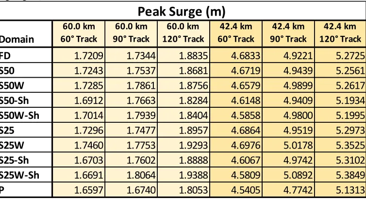
As expected, the smaller, more intense storms caused greater peak elevations (Table 3-1, right, gold) than the larger, less intense storms (Table 3-1, left, pale gold). For storms with a Rm of 42.4 km, the average peak elevation at Recording Station 36 was 4.95 m above MSL, and it was 1.78 m above MSL for storms with a Rm of 60.0 km (calculated using values in Table 3-1).
Table 3-1: Maximum elevation (meters) in each domain during each storm at Recording Station 36, colors indicating increase in elevation with decreasing storm size. The larger (Rm = 60.0 km), more diffuse storms produced lower peak elevations (left, pale gold). The smaller (Rm = 42.4 km), more intense storms produced higher peak elevations (right, gold).
For each storm size, peak elevation increased with increasing track angle for the three tracks considered (60°, 90°, and 120°) (Table 3-2). The following percent change values were calculated using elevations from Table 3-2. For the larger (Rm = 60.0 km), less intense storms, the storm approaching from the southwest (120° track) caused a mean increase in peak elevation of 6.57% compared with the shore-normal approach, and the storm approaching from the
southeast (60° track) caused a mean decrease in peak elevation of 3.17%. For the smaller (Rm = 42.4 km), more intense storms, the storm approaching from the southwest caused a similar mean increase in peak elevation (6.20%) from the shore-normal approach as the larger storm.
However, the smaller storm approaching from the southeast caused a larger decrease in peak elevation (6.57%) than the large storm approaching from the southeast. It is likely that the substantial setdown that occurred prior to the arrival of peak surge during the smaller, more powerful storm contributed to the decreased peak surge level. The impact of landfall direction on peak elevation found in this study (an increase in peak surge for track angles greater than 90° and a decrease in peak surge for track angles less than 90°) is consistent with the findings of Irish et al. (2008) who found that all storm tracks with more westerly headings (45°-75°) produced smaller surges than the due north (90°) track for both moderately and mildly sloping bottoms. For the most mildly sloping bottom (1:10,000), storms with more easterly headings (105°-150°)
Domain 60.0 km 60° Track 60.0 km 90° Track 60.0 km 120° Track 42.4 km 60° Track 42.4 km 90° Track 42.4 km 120° Track
FD 1.7209 1.7344 1.8835 4.6833 4.9221 5.2725 S50 1.7243 1.7537 1.8681 4.6719 4.9439 5.2561 S50W 1.7285 1.7861 1.8756 4.6579 4.9899 5.2617 S50-Sh 1.6912 1.7663 1.8284 4.6148 4.9409 5.1934 S50W-Sh 1.7014 1.7939 1.8404 4.5858 4.9800 5.1995 S25 1.7296 1.7477 1.8957 4.6864 4.9519 5.2973 S25W 1.7460 1.7753 1.9293 4.6976 5.0178 5.3525 S25-Sh 1.6703 1.7602 1.8888 4.6067 4.9742 5.3102 S25W-Sh 1.6691 1.8064 1.9388 4.5809 5.0892 5.3849 P 1.6597 1.6740 1.8053 4.5405 4.7742 5.1313