Harpenden, Herts, AL5 2JQ
Telephone: +44 (0)1582 763133 Web: http://www.rothamsted.ac.uk/
Rothamsted Research is a Company Limited by Guarantee Registered Office: as above. Registered in England No. 2393175. Registered Charity No. 802038. VAT No. 197 4201 51. Founded in 1843 by John Bennet Lawes.
Rothamsted Repository Download
A - Papers appearing in refereed journals
Foster, S. P., Denholm, I., Thompson, R., Poppy, G. M. and Powell, W.
2005. Reduced response of insecticide-resistant aphids and attraction of
parasitoids to aphid alarm pheromone; a potential fitness trade-off.
Bulletin of Entomological Research. 95 (1), pp. 37-46.
The publisher's version can be accessed at:
•
https://dx.doi.org/10.1079/BER2004336
The output can be accessed at:
https://repository.rothamsted.ac.uk/item/895y4
.
© 9 March 2007, Cambridge University Press (CUP).
Biometrics 62, 392–401
June 2006
DOI: 10.1111/j.1541-0420.2005.00500.x
The Analysis of Longitudinal Data Using Mixed Model L-Splines
Sue J. Welham,1,∗ Brian R. Cullis,2 Michael G. Kenward,3 and Robin Thompson1
1Rothamsted Research, Harpenden AL5 2JQ, U.K.
2Wagga Agricultural Institute, Wagga Wagga, NSW 2650, Australia 3London School of Hygiene and Tropical Medicine, London WC1E 7HT, U.K.
∗email:[email protected]
Summary. L-splines are a large family of smoothing splines defined in terms of a linear differential operator.
This article develops L-splines within the context of linear mixed models and uses the resulting mixed model L-spline to analyze longitudinal data from a grassland experiment. In the spirit of time-series analysis, a periodic mixed model L-spline is developed, which partitions data into a smooth periodic component plus smooth long-term trend.
Key words: Longitudinal data; L-splines; Mixed models; Residual maximum likelihood; Smoothing splines.
1. Introduction
This article develops mixed model L-splines, motivated by an experiment to investigate grassland response to different treatment regimes. Within this experiment, data on available pasture dry matter (termed food on offer) were collected from individual plots over 4 years, which showed a strong seasonal pattern as well as longer-term trend. The aim was to parti-tion the data for each treatment into periodic and nonperiodic components, both modeled as a continuous function of time. As the plot profiles across time did not correspond to any sim-ple parametric form, smoothing splines provided a convenient method of curve fitting, which could be built into a standard linear mixed model for longitudinal data.
Cubic smoothing splines were introduced into the mixed model setting by Wang (1998), Zhang et al. (1998), Brumback and Rice (1998), and Verbyla et al. (1999), who all used the mathematical equivalence between the penalized sum of squares used to fit a cubic spline and best linear unbiased predictor (BLUP) estimation in a particular mixed model for a given smoothing parameter. Within this mixed model, the cubic spline corresponds to fitting a model with linear trend plus a set of random covariates whose covariance matrix is known apart from a scaling constant, called the smoothing variance component. In addition, residual maximum likeli-hood (REML) estimation of the smoothing variance compo-nent in the linear mixed model is equivalent to the gener-alized maximum likelihood method for smoothing parameter estimation of Wahba (1990). Within the linear mixed model context, a cubic spline can be included within a general treat-ment structure and fitted at different levels of the structure, for example, as a common spline across all treatments, or as separate splines for different treatment combinations (Verbyla et al., 1999). Additional random terms can easily be added to the model to account for all sources of variation in the data. Other types of smoothing splines have also been used
within mixed models, with the same motivation of building nonparametric terms into a general and flexible family of mod-els. Eilers and Marx (1996) developed P-splines, which used a B-spline basis with an approximate discrete penalty and a reduced set of knots. Although they fitted these models us-ing cross-validation, Eilers noted in the discussion of Verbyla et al. (1999) that P-splines could also be fitted as mixed model splines with the smoothing parameter estimated by REML, as demonstrated by Currie and Durban (2002). Parise et al. (2001) proposed a slightly different mixed model spline, us-ing truncated power basis functions for polynomial splines with an identity penalty matrix, and called these functions penalized splines. These spline models also used a reduced set of knots and the smoothing parameter was estimated us-ing REML. Wand (2003) gives a general review of penalized spline models and some extensions.
In the mixed model context the cubic spline is partitioned into a fixed linear component plus a random component, with zero expectation, representing smooth deviations about the linear trend. Although the standard interpretation of a spline is as a single smooth trend, we find this partition useful to in-terpret the difference between L-splines with polynomial and periodic core functions. For a given value of the smoothing pa-rameter, the fitted cubic spline is determined by minimizing the residual sum of squares for the model subject to a penalty consisting of the integrated squared second derivative of the fitted curve, i.e., of deviations from linear trend, scaled by the smoothing parameter. However, in many examples the under-lying trend is not linear. In the grassland experiment consid-ered later, the underlying pattern is a seasonal cycle with some linear trend, which does not reflect the implicit assump-tions of the mixed model cubic spline. It then seems more natural to use L-splines that fit an appropriate underlying form plus smooth deviations about this underlying form. The amount of smoothing is controlled by a penalty constructed
to penalize departures from the appropriate underlying form. The theory behind L-splines is given briefly by Wahba (1990), and more accessibly by Gu (2002) or Ramsay and Silverman (1997). Ramsay and Dalzell (1991), Ramsay and Silverman (1997), and Heckman and Ramsay (2000) all used L-splines in preference to cubic splines where the underlying form of the data was not linear, and particularly for periodic data.
In this article, we show that L-splines can be fitted as mixed models and extend the model to partition deviations from the underlying form into periodic and nonperiodic components. We demonstrate our approach using mixed model L-splines to model data from the grassland experiment described in Section 2. Section 3 gives a brief overview of the construction of L-splines, and Section 4 shows the mixed model form of the L-spline, extends the definition to a reduced set of knots, and evaluates the performance of an L-spline, in terms of mean squared error of prediction, in a small simulation study. In Section 5, the development of a periodic L-spline term is de-scribed and its performance is evaluated. Finally, in Section 6 the methods are used to analyze data from the grassland ex-periment and obtain results, with discussion in Section 7.
2. Grassland Experiment
The data that motivated the analysis in this article were kindly provided by D. L. Garden of NSW DPI (Canberra) and arose from a grassland experiment designed to investi-gate the effects of superphosphate application and grazing on
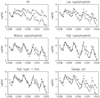
Figure 1. Log(FOO) measurements (as log kg dry matter per hectare) across time for each plot of each treatment (× =
replicate 1,◦= replicate 2) with predictive component of the final model from Table 3 (solid line = replicate 1, dashed line = replicate 2).
394 Biometrics, June2006
3. L-Splines
Suppose we have datay(n×1) and an explanatory variable
xobserved at unique valuesx1,x2,. . .,xn in the range [a,b].
An L-spline is defined in terms of the underlying form of the data, described by a set of core functions{fj;j= 1,. . .,m},
and associated linear differential operatorLof orderm, which annihilates the core functions, i.e.,Lf= 0 if and only iffis a linear combination of thefj orf≡0. For example, the linear
differential operatorL = D4 +ω2D2 annihilates the set of core functions
f1(t) = 1; f2(t) =t; f3(t) = cos(ωt); f4(t) = sin(ωt).
The polynomial splines (of odd degreek = 2m −1) form a subset of L-splines whereL =Dm for positive integersm. In
general, the functionsfmay depend on unknown parameters. In this article, we assume that all such parameters (e.g., the period parameterω) are known.
For a single spline term, we fit a model
y=g+e,
wheregis the realization of an unknown smooth functiong(t) at the data pointsx, i.e.,g=g(x), andeis a vector of errors withe∼ N(0,σ2R), for some general covariance matrixR. The L-spline is the functiong(t) that minimizes the penalized sum of squares,
(y−g)R−1(y−g) +λ
b
a
[Lg(s)]2ds, (1)
for a given value ofλ, the smoothing parameter. The smooth-ing parameter determines the balance between fidelity to the data (measured by the first term, a residual sum of squares) and fidelity to the underlying form (measured by the second term). Ramsay and Silverman (1997, Section 15.2) prove that, for any basis{fj;j= 1,. . .,m}for the set of core functions,
the functiong minimizing the penalized sum of squares (1) has the form
g(t) =
m
j=1
τjfj(t) + n
i=1
cik2(xi, t),
where k2 is the reproducing kernel function for a subspace defined in terms of the operator L and a set of boundary conditions. We used initial value boundary constraints (see Ramsay and Silverman, 1997, Section 13.5.1). Ramsay and Silverman (1997, Section 15.3) further show that equation (1) can then be reexpressed as
(y−Xτ−Kc)R−1(y−Xτ−Kc) +λcKc, (2) where [X]ij =fj(xi) fori= 1,. . .,n,j = 1,. . .,m, [K]ij =
k2(xj,xi) for i,j = 1,. . .,n, τ = (τ1,. . .,τm), and c =
(c1,. . .,cn). Gu (2002) shows that the symmetric matrixK
is nonnegative definite. Heckman and Ramsay (2000) and Dalzell and Ramsay (1993) give recipes for constructing re-producing kernel functionsk2. ForL =ω2D2 +D4 and a= 0 the reproducing kernel functionk2can be written as
k2(xi, t) =
1
ω6
ω2t2
6 (3xi−t)−(xi−t) +xicos(ωt)
+tcos(ωxi)−
1
ωsin(ωt)−
1
ωsin(ωxi)
+1
2tcos[ω(xi−t)] + 1
ωsin[ω(xi−t)]
− 1
2ωcos(ωxi) sin(ωt)
for t < xi
k2(xi, t) =
1
ω6
ω2x2
i
6 (3t−xi)−(t−xi) +tcos(ωxi)
+xicos(ωt)−
1
ωsin(ωxi)−
1
ωsin(ωt)
+1
2xicos[ω(t−xi)] + 1
ωsin[ω(t−xi)]
− 1
2ωcos(ωt) sin(ωxi)
for xi< t. (3)
Consider functions defined piecewise on [xi−1,xi] as β1i+β2it+β3it2+β4it3+β5icosωt
+β6isinωt+β7itcosωt+β8itsinωt, (4)
for xi−1 ≤ t ≤ xi,i = 1,. . .,n (x0 = a), with the require-ment that the overall function is continuous and differentiable up to order 6 (= 2m − 2) at the knots. It is straightfor-ward to show that the functions defined in equation (3) are of this form. Together with the global functions {1,t,t2,t3, cos(ωt), sin(ωt),tcos(ωt),tsin(ωt)}, these functions span the space of six-times differentiable functions that are piecewise (between knots) of the form (4), i.e., periodic with linearly varying amplitude and with added cubic trend.
4. L-Spline Mixed Models
The L-spline is fitted to the datayby finding the coefficient values ˆτ and ˜cthat minimize the penalized sum of squares (2) for a given value of the smoothing parameterλ. Minimization of equation (2) requires solution of the equations
XR−1X XR−1K KR−1X KR−1K+λK
ˆ
τ
˜
c =
XR−1y KR−1y .
These equations contain m implicit constraints that can be expressed asX˜c=0(see, for example, Wahba, 1990, equa-tion 1.3.17). This property has the consequence that the fitted spline takes the underlying form outside the range of the data, i.e.,Lg(t) = 0 fort<x1 ort>xn. Following the terminology
of polynomial splines, we call this a natural L-spline. For con-venience, we make this implicit constraint on the parameter estimates explicit in our model as Xc =0. The constraint
Xc=0implies c=Cδ for some vectorδ of lengthn− m
where C is any n × n − m matrix C of full column rank such that XC = 0. Inserting this reparameterization into the penalized sum of squares (2) gives
(y−Xτ−Zδ)R−1(y−Xτ−Zδ) +λδH−1δ,
where Z = KC, H−1 =CKC, and it can be shown that
XR−1X XR−1Z
ZR−1X ZR−1Z+λH−1 ˆ
τ
˜
δ =
XR−1y
ZR−1y , which are the mixed model equations for the model
y=Xτ+Zδ+e,
where Xτ represents the core functions as fixed terms in the model, Zδ represents the constrained basis of re-producing kernel functions as a random model term, vec-tor e represents a residual term, and e∼N(0, σ2R),δ∼
N(0, σ2
sH),cov(δ,e) =0, λ=σ2/σ2s.
As for cubic splines (Verbyla et al., 1999), the fitted L-spline can then be calculated as a BLUP from this mixed model for a given value of the smoothing parameter. The smoothing pa-rameter can either be considered fixed at some predetermined value or estimated, via the L-spline variance componentσ2
s,
as part of the variance model using REML estimation. In this article, we use REML estimation of smoothing parameters, as used by Verbyla et al. (1999) for cubic smoothing spline models. The extension to include additional fixed or random terms is achieved by simply adding these terms into the mixed model.
It is often convenient in practice to transform to indepen-dent random effects u, where u =H−1/2δ and the random design matrixZis replaced byZH1/2 with var(u) =σ2
sIn−m.
The mixed model L-spline can then easily be fitted by most standard mixed model software. We write this final model as
y=Xτ+Zuu+e,
whereZu=ZH1/2with other terms as above. For
interpreta-tion, it is also advantageous to make the spline design matrix
Zuorthogonal to the fixed effect design matrixX.
The change in logRL, the logarithm of the REML likelihood function, on adding the random L-spline term to the model containing the core functions, i.e., testing for a zero variance component, can be used to investigate whether there is evi-dence of deviations from the underlying form (Guo, 2002b). As a likelihood ratio test with the variance component con-strained to remain positive, the asymptotic distribution of 2× the change in logRL is a 50:50 mixture of aχ2
0and aχ21 distri-bution under the null hypothesis (Stram and Lee, 1994). How-ever, Crainiceanu and Ruppert (2004) showed that in many examples this approximation was very poor, and developed a better approximation for models with a single variance com-ponent in addition to the residual variance. Crainiceanu et al. (2005) suggested parametric bootstrap evaluation of the null distribution for more complex variance models. Zhang and Lin (2003) specified a score test for the smoothing parameter.
4.1 Reduced Knot Set
For data sets with a large number of distinct covariate val-ues, or with several spline terms in the model, the L-spline mixed model may generate a large number of random spline effects with a dense design matrixZu. Solution of the mixed
model equations may then require a large amount of com-puter workspace and processing time. Both can be reduced by using a (relatively) small number of knots, rsay, defined at distinct values t = (t1,t2,. . .,tr) with a < t1 < · · · <
tr< b. Our development here is similar to that of Parise et al.
(2001) and Wand (2003), who used a reduced number of knots
in generating polynomial spline basis functions as a low-rank approximation to the full basis.
The set ofrL-spline basis functions is generated ask2(ti,·)
fori= 1,. . .,r, using the reduced set of knots,t. The L-spline function then takes the form
g(t) =
m
j=1
τjfj(t) + r
i=1
cik2(ti, t),
and the penalized sum of squares corresponding to this func-tion is written as
(y−g)R−1(y−g) +λ
b
a
[Lg(s)]2ds
= (y−Xτ−Kxtc)R−1(y−Xτ−Kxtc) +λcKttc,
where now [Ktt]ij = k2(tj,ti), i,j = 1,. . .,r, because the
penalty term is defined in terms of therbasis functions eval-uated at the knots, [Kxt]ij = k2(tj,xi), i = 1,. . .,n,j =
1,. . .,r, gives the value of therbasis functions at then covari-ate values,τ = (τ1,. . .,τm) andc= (c1,. . .,cr). In order to
retain the natural spline property achieved for L-splines with knots at all data points, we explicitly impose the constraint
Xtc=0, where [Xt]ij=fj(ti),i= 1,. . .,r,j = 1,. . .,m, to
get the amended penalized sum of squares
(y−Xτ−KxtCtδ)R−1(y−Xτ−KxtCtδ) +λδH−tt1δ,
(5)
whereCt is anr× r−mmatrix defined such thatXtCt = 0,H−1
tt =CtKttCt, andδ = (δ1,. . .,δr−m). Minimizing (5)
yields mixed model equations for the model
y=Xτ+Ztδ+e, (6)
whereZt =KxtCt andδ∼N(0,σ2s Htt).
The fitted spline, estimated smoothing parameter, and logRL are not invariant to the reduced set of knots chosen, although the fitted spline is usually similar at the data points. In addition, the reduced knot L-spline is no longer the func-tion that produces the overall minimum of the penalized sum of squares (1) and care is required to ensure that the fitted spline is not sensitive to the knots used. Ruppert (2002) dis-cusses choice of knots in the penalized spline context.
Verbyla et al. (1999), Wang (1998), and Brumback and Rice (1998) all utilized a hierarchical decomposition in their cubic spline mixed models by decomposing individual treat-ment splines into an overall spline, main effect splines, and interaction splines. In addition, Verbyla et al. (1999) used subject-specific splines to model the profile of individual sub-jects over time. A similar model was proposed by Guo (2002a). An exactly analogous decomposition can be used for L-spline mixed models.
4.2 Evaluation of L-Splines versus Cubic Splines
396 Biometrics, June2006
that vary between years. In addition, the long-term trend may change according to grazing pressure and treatment regimes. To represent these features we simulated monthly data across 5 years, using known curves of the form
cjk(t) =s1jk(t) + (s2jk(t)−0.03)(t−30.5)
+ [0.5 +s3jk(t)] sin[ωjk(t)(t+s4jk(t))], (7)
where ωjk(t) = 2π/(12 + s5jk(t)), for j = 1,. . ., 9, k =
1,. . ., 10. The average amplitude and linear trend were chosen to match that of the log(FOO) data from the grassland exper-iment. The functionssijk(t) were generated from independent
realizations of an N(0, 1) random walk, smoothed using a cubic spline with four effective degrees of freedom, then stan-dardized to a predetermined rangerij(sorij= 0⇒sijk(t)≡0).
This generated smooth deviations in trend and in amplitude, length, and timing of the annual cycle. Nine combinations (j) of range values, shown in Table 1, were investigated. For each set, realizations sijk(t) were generated for k = 1,. . ., 10 and
used to form a set of representative curves cjk(t). For each
curvecjk(t), 500 sets of data were independently generated as yjkl =cjk(x) +ejkl,l= 1,. . ., 500, withx= (1,. . ., 60),ejkl ∼ N(0,σ2I
60). Two values of the residual varianceσ2 were as-sessed, with σ2 equal to 0.01 or 0.001. Each data set was modeled using a cubic smoothing spline, a partial cubic spline (PCS) consisting of the cubic smoothing spline plus additional fixed periodic functions sin(ωt) and cos(ωt), and an L-spline withL =ω2D2 +D4. The splines were all fitted as mixed model splines using REML estimation of variance parameters, using several starting values to ensure that a global optimum was reached. The fit of the models to the data was evaluated using the average mean squared error of prediction (MSEP)
Table 1
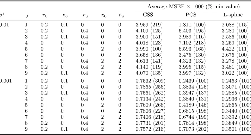
Average MSEP across5000data sets(model7)for a cubic smoothing spline(CSS),partial cubic spline
(PCS),and L-spline model(withL=D4 +ω2D2). Average MSEP values are also shown as a percentage
of minimum value for each row.
Average MSEP×1000 (% min value)
σ2 j r
1j r2j r3j r4j r5j CSS PCS L-spline
0.01 1 0.2 0.1 0 0 0 3.959 (219) 1.811 (100) 2.088 (115) 2 0.2 0 0.4 0 0 4.109 (125) 6.403 (195) 3.280 (100) 3 0.2 0.1 0.4 0 0 3.909 (151) 2.989 (116) 2.586 (100) 4 0 0 0.4 0 0 4.018 (123) 7.102 (218) 3.259 (100) 5 0 0 0 2 0 3.990 (100) 6.593 (165) 4.422 (111) 6 0 0 0 0 2 3.658 (136) 3.475 (130) 2.676 (100) 7 0 0 0.4 2 2 4.613 (141) 4.323 (132) 3.278 (100) 8 0.2 0 0.4 2 2 4.140 (119) 3.995 (115) 3.481 (100) 9 0.2 0.1 0.4 2 2 4.070 (135) 3.997 (132) 3.022 (100) 0.001 1 0.2 0.1 0 0 0 0.7532 (309) 0.2439 (100) 0.2463 (101)
2 0.2 0 0.4 0 0 0.7865 (256) 0.3834 (125) 0.3071 (100) 3 0.2 0.1 0.4 0 0 0.7561 (262) 0.3947 (137) 0.2885 (100) 4 0 0 0.4 0 0 0.7134 (242) 0.3840 (131) 0.2936 (100) 5 0 0 0 2 0 0.7609 (266) 0.4189 (146) 0.2865 (100) 6 0 0 0 0 2 0.7806 (227) 0.6815 (198) 0.3440 (100) 7 0 0 0.4 2 2 0.7406 (218) 0.6744 (199) 0.3392 (100) 8 0.2 0 0.4 2 2 0.7731 (201) 0.7614 (198) 0.3849 (100) 9 0.2 0.1 0.4 2 2 0.7572 (216) 0.7073 (202) 0.3501 (100)
1 10
10
k=1 1 500
500
l=1
[cjk(x)−c˜jkl(x)][cjk(x)−˜cjkl(x)],
where ˜cjkl(t) is the relevant fitted spline for datayjkl. Table 1
shows the average MSEP for each set of parameters. Forj= 1, where deviations from the annual cycle consisted only of changes in long-term trend, the PCS had the smallest MSEP value. In all but one case, where variation was introduced into the periodic cycle the L-spline had the smallest MSEP. The relative improvement for the L-spline increased forσ2 = 0.001 and then the PCS always had smaller MSEP than the cubic spline alone. For σ2 = 0.01 the cubic spline sometimes had a smaller MSEP value than the partial spline, and for
j= 5 was smaller than both the cubic smoothing spline and L-spline. In this case, both the PCS and L-spline occasion-ally oversmoothed the data, using variance components close to zero and inflating the overall MSEP. In contrast the cu-bic smoothing spline consistently overfitted the data, severely underestimating the residual variance.
5. Modeling the Within-Year Component: Periodic Splines
and Sowers (2000) who used the full (nonnatural) basis for a cubic smoothing spline and applied periodic constraints. Clearly, fitting a full additional L-spline would lead to iden-tifiability problems. We resolve this by fitting a single set of core functions with two sets of basis functions: the natural L-spline functions derived earlier, and a set derived from the full basis but constrained to be periodic. ForL=D4+ω2D2 withm= 4 andpknots (t1,. . .,tp) within the period [0,T], T = 2π/ω, we construct the periodic component from a set ofpbasis functionsk2(ti;t), defined using equation (3),
aug-mented by the m noncore global basis functionsl1(t) = t2,
l2(t) =t3,l3(t) =tcos(ωt),l4(t) =tsin(ωt). Define
gd(t) = p
i=1
dik2(ti, t) + m
j=1
dp+jlj(t),
with associated penalty matrixKa constructed such that for d= (d1,. . .,dp+m)
dKad=
T
0
[Lgd(s)]2ds.
Periodic constraints are applied as Gd = 0 where G is a (p+m)×(2m−1) matrix
Gij=
k2(j−1)(ti, T)−k2(j−1)(ti,0) i= 1, . . . , p,
l(pj+−i1)(T)−l(pj+−i1)(0), i= 1, . . . , m,
forj=1, . . . , 2m−1 with 2m−1 constraints applied to ensure the same degree of continuity as in the underlying basis func-tions. It follows thatd=Cpυfor a (p+m)×(p−m+ 1)
matrix Cp such thatGCp =0. The model (6) is extended
to include a periodic component
y=Xτ+Ztδ+Zpυ+e,
withZp=KxpCp, whereKxp evaluates thep+mnoncore
basis functions at the covariate values, andυ∼N(0,σ2
pHpp)
forH−1
pp=CpKaCpwith cov (v,δ) = cov (v,e) =0.
Table 2
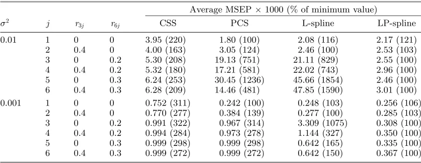
Average MSEP across5000data sets(model8)for a cubic smoothing spline(CSS),partial cubic spline
(PCS),L-spline, and L-spline with additional periodic spline(LP-spline). Average MSEP values are also shown as a percentage of the minimum value for each row.
Average MSEP×1000 (% of minimum value)
σ2 j r
3j r6j CSS PCS L-spline LP-spline
0.01 1 0 0 3.95 (220) 1.80 (100) 2.08 (116) 2.17 (121) 2 0.4 0 4.00 (163) 3.05 (124) 2.46 (100) 2.53 (103) 3 0 0.2 5.30 (208) 19.13 (751) 21.11 (829) 2.55 (100) 4 0.4 0.2 5.32 (180) 17.21 (581) 22.02 (743) 2.96 (100) 5 0 0.3 6.24 (253) 30.45 (1236) 45.66 (1854) 2.46 (100) 6 0.4 0.3 6.28 (209) 14.46 (481) 47.85 (1590) 3.01 (100) 0.001 1 0 0 0.752 (311) 0.242 (100) 0.248 (103) 0.256 (106)
2 0.4 0 0.770 (277) 0.384 (139) 0.277 (100) 0.285 (103) 3 0 0.2 0.991 (322) 0.967 (314) 3.309 (1075) 0.308 (100) 4 0.4 0.2 0.994 (284) 0.973 (278) 1.144 (327) 0.350 (100) 5 0 0.3 0.999 (298) 0.999 (298) 0.642 (165) 0.335 (100) 6 0.4 0.3 0.999 (272) 0.999 (272) 0.642 (150) 0.367 (100)
5.1 Evaluation of Extended Model with Periodic Spline Component
The simulation study of Section 4.2 was modified to investi-gate the performance of the periodic spline component, again using curves of relevance to the log(FOO) data from the grass-land experiment. Using the notation of Section 4.2, curves were generated as
cjk(t) =s1jk(t) + (s2jk(t)−0.03)(t−30.5)
+ (0.5 +s3jk(t)) sin(ωt) + r6jsin(2ωt), (8)
where ω= 2π/12 forj = 1,. . ., 6,k = 1,. . ., 10. The func-tionss1jk(t),s2jk(t) usedr1j= 0.2,r2j= 0.1 for alljto provide
smooth nonlinear trend. The amplitude of the underlying pe-riodic cycle was either kept constant (r3j = 0) or allowed to
vary (r3j= 0.4). Extra periodic components were added to the
curve as sin(2ωt) to mimic the extra periodic pattern found in the log(FOO) data, and as a component orthogonal to the underlying periodic function. The effect of adding this term was assessed using coefficientr6j = 0, 0.2, or 0.3. For each
curvecjk(t), 500 sets of data were generated for σ2 equal to
0.01 or 0.001. Each data set was modeled using the splines assessed in Section 4.2 and an L-spline with additional peri-odic L-spline, both usingL=ω2D2 +D4. Table 2 shows the average MSEP for each set of parameters. In every case where
r6j >0, the MSEP for the model including the periodic spline
398 Biometrics, June2006
coefficient r6j increased, but both performed badly in some
cases. The presence of the periodic spline in the model guards against this problem.
The ability of the periodic spline to separate periodic de-viations from long-term trend was evaluated by examining the periodic spline and long-term L-spline components of the fitted model, and residuals from the fitted model. For the long-term L-spline component and residuals, each series was detrended (using a smoothing spline with 4 degrees of free-dom) and then the periodic component extracted by fitting a linear model with effects for the 12 months of the year. The sum of squares accounted for by month was used as a mea-sure of periodic trend in each component. The variation in the periodic spline was measured by its total sum of squares. The total periodic variation was measured by the total of the three sums of squares. Forr6j >0, the proportion of periodic
variation accounted for by the periodic spline increased asr6j
increased and asσ2 decreased, and was in the range 88–97%, with 1–8% accounted for in the long-term L-spline and 0–4% in the residual.
6. Analysis of the Grassland Experiment
The FOO data were analyzed using a logarithmic transforma-tion to stabilize the variance of the data. The L-spline with core functions{1,t, sin(ωt), cos(ωt)}was used to model long-term trend, with an additional set of periodic basis functions as described in Section 5. The structure of the experiment can be written symbolically (using the notation of Wilkinson and Rogers, 1973) as (rep/plot)∗sample, where “∗” is a crossing operator (i.e.,rep∗sample=rep+sample+rep.sample), “/” is a nesting operator (i.e.,rep/plot=rep +rep.plot), “.” de-notes an interaction,repindicates replicates in the design,plot
indicates plots within replicates, andsampleindicates the 32 sample dates. The treatment structure can be written astrt∗ sample, wheretrtlabels the six fertilizer treatments. We wish to model the pattern across sample dates in terms of the un-derlying variable time, decomposing the term into linear trend
lin(t), sine/cosine periodic termsin(ωt),cos(ωt), L-spline de-viations lspl(t), and periodic L-spline deviations pspl(t). To complete this decomposition, we need the residual (or lack of fit) term, sample, to represent pattern not accounted for by other terms, which can be separated from random variation due to the replicate plots measured at each sample date. The lack-of-fit term was fitted as a random term with independent errors, analogous to the usual lack-of-fit term in a regression model. The full model is shown in Table 3. In the bottom stratum, Rep.Plot.Sample, residual error could be considered as a composite of variation due to intrinsic plot effects on pas-ture growth, which would be correlated over time, and ran-dom measurement error. This composite structure was decom-posed into separate independent and correlated components, with correlation within plots between samples ddays apart modeled asφd, with a common parameter 0< φ < 1
esti-mated across all plots. Eight values were chosen to represent typical sample dates within years. These eight points were used as knots for the periodic spline, and the corresponding 32 dates across the 4 years were used as knots for the nonpe-riodic L-spline.
Model selection started with the full model shown in Table 3. Variance components relating to random terms were
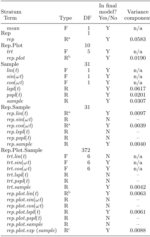
Table 3
Structural decomposition showing full model for log(FOO)
data, terms indicated as fixed(F)or random(R). Degrees of freedom(DF) shown for each stratum and for fixed terms. Scaled estimated variance components are shown for random
terms retained in the final model.
In final
Stratum model? Variance
Term Type DF Yes/No component
mean F 1 Y n/a
Rep 1
rep Ra Y 0.0583
Rep.Plot 10
trt F 5 Y n/a
rep.plot Rb Y 0.0190
Sample 31
lin(t) F 1 Y n/a
sin(ωt) F 1 Y n/a
cos(ωt) F 1 Y n/a
lspl(t) R Y 0.0617
pspl(t) R Y 0.0201
sample R Y 0.0307
Rep.Sample 31
rep.lin(t) Ra Y 0.0097
rep.sin(ωt) R N –
rep.cos(ωt) Ra Y 0.0039
rep.lspl(t) R N –
rep.pspl(t) R N –
rep.sample R Y 0.0040 Rep.Plot.Sample 372
trt.lin(t) F 6 N n/a
trt.sin(ωt) F 6 Y n/a
trt.cos(ωt) F 6 Y n/a
trt.lspl(t) R N –
trt.pspl(t) R N –
trt.sample R Y 0.0042
rep.plot.lin(t) Rb Y 0.0063
rep.plot.sin(ωt) R N –
rep.plot.cos(ωt) R N –
rep.plot.lspl(t) R Y 0.0061
rep.plot.pspl(t) R N –
rep.plot.sample R N –
rep.plot.exp(sample) Rc Y 0.0088 aIndicates correlated terms fitted using rank 1 model.
bIndicates correlated terms fitted using unstructured model. cexp(·) indicates exponential correlation model.
Table 4
LogRL for models for log(FOO)data. The final fixed/random models refer to Table3. LogRL for model14is not comparable with other models as a different set of fixed terms was fitted.
Number of Change in variance logRL from Model Terms included in model LogRL parameters model (2)
1 All fixed and random terms in Table 3 466.99 23 0.72 2 All fixed terms, final random model 466.27 14 – 3 Model (2) without termpspl(t) 463.04 13 −3.23 4 Model (2) without termrep.plot.lspl(t) 460.48 13 −5.78 5 Model (2) without termlspl(t) 463.71 13 −2.56 6 Model (2) without termtrt.sample 456.13 13 −10.14 7 Model (2) without termrep.sample 449.04 13 −17.23 8 Model (2) without termsample 450.76 13 −15.51
9 Model (2) without termrep 462.12 13 −4.15
10 Model (2) without termrep.lin(t) 463.79 13 −2.48 11 Model (2) without termrep.cos(t) 458.45 13 −7.82 12 Model (2) without termrep.plot 452.82 12 −13.45 13 Model (2) without termrep.plot.lin(t) 453.13 12 −13.14
14 Final fixed and random models 484.27 14 –
there were only two reps, a full unstructured model could not be fitted between termsrep,rep.lin(t), andrep.cos(ωt), but a rank 1 model with correlation 1 increased logRL compared to independent terms. A correlation of 0.89 was estimated be-tween the plot intercept (rep.plot) and linear (rep.plot.lin(t)) terms. The REML estimate of ˆφ= 0.997 was equivalent to a correlation of 0.35 between samples taken 45 days apart from the same plot. Once the final variance model was estab-lished, the fixed model was simplified using Wald tests in a backward selection strategy, respecting marginality. The final fixed model allowed for a separate intercept and periodic pat-tern for each fertilizer treatment, with a common linear trend. GenStat (Payne, 2003) and ASREML (Gilmour et al., 2002) were used for the analysis.
The REML estimates of the variance components are shown in Table 3 multiplied by the mean value of the diagonal of the matrix ZiZi in order to indicate the average
contri-bution of the term to the variance of a data value. Variation due to the random regressions on rep/(lin(t) + cos(t)) and
rep.plot/lin(t) was relatively large due to differences between replicates (see Figure 1). As the stocking rate was the same for both replicates, the replicate with less initial FOO would be expected to show a greater decline, and hence positive correlation between intercept and linear terms. As there were also initial differences in available pasture between replicate plots for each treatment, and as stocking rate was changed on plots according to the treatment, a similar correlation structure with highly correlated intercept and linear terms was observed for plots within replicates. The variance com-ponents corresponding to overall spline and lack-of-fit terms also made a significant contribution to the variation of the data compared to the residual component. The presence of the periodic L-spline (pspl(t)) indicated a common seasonal pattern of deviations about the underlying model for all treat-ments. However, the nonperiodic L-spline (lspl(t)) and lack-of-fit (sample) terms had larger variance components, indicating substantial nonperiodic smooth trend over time with some
lack of fit. There was no evidence that separate splines were required for different fertilizer treatments, although the small
rep.plot.lspl(t) term indicated differences in long-term patterns between plots. There was also some lack of fit to individual treatment profiles, indicated by thetrt.sampleterm.
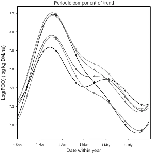
Figure 2. Total periodic component of final model
400 Biometrics, June2006
Figure 1 presents the log-transformed data with fitted curves calculated by excluding all lack-of-fit terms and the residual, as these terms represent unpredictable noise. There was good agreement between the data and the fitted curves. The nonperiodic trend over time did not depend on treat-ment and showed a steady decrease in FOO over time af-ter the first year. Figure 2 shows the periodic component of the trend for each treatment, calculated from the treatment-specific constant, sine/cosine, and common periodic L-spline terms. Differences in phase and amplitude arise solely from the fixed terms in the model and it is clear that amplitude increased with superphosphate levels. However, applying su-perphosphate with lime or sewage ash appeared to provide extra herbage mass during the autumn and winter (May– August). The deviation away from the underlying sine/cosine shape was introduced by the periodic L-spline component. The main influence of the periodic L-spline was to sharpen the main peak during November and December, and to in-troduce some regrowth in May and June. This inin-troduced an extra bump into the pattern for lower levels of superphos-phate, and a reduced rate of decrease for higher levels. This regrowth was present in the raw data (Figure 1) but could not be modeled by the underlying fixed model.
7. Discussion
We have shown that L-splines with linear parameters in the core functions can be implemented within mixed models in a similar manner to cubic smoothing splines, and can be used to give ANOVA-type decompositions of the treatment structure. The extension to a periodic L-spline term is help-ful in giving a familiar decomposition into periodic and non-periodic components of the trend. The model with the pe-riodic L-spline allows an explicit prediction of the shape of the periodic component; in the grassland example this can be used to predict the pattern of log(FOO) in an average year.
Heckman and Ramsay (2000) showed that use of the ap-propriate L-spline required a smoother with fewer degrees of freedom than a cubic spline, and Ramsay and Dalzell (1991) argued that the partitioning of the function space into orthogonal subspaces (with respect to the inner prod-uct) was in itself desirable. Our small simulation showed that a mixed model L-spline with core functions accounting for a linear trend with a periodic cycle can perform better than either cubic splines or PCS in terms of squared error of prediction when there are perturbations in the periodic cycle. Further work is required to establish the full range of conditions under which mixed model L-splines could be recommended.
Acknowledgements
We gratefully acknowledge funding from the Grains Research and Development Corporation of Australia for this work, and thank D. L. Garden for permission to use the data from the grassland experiment and advice on the interpretation of the analysis.
References
Brumback, B. A. and Rice, J. A. (1998). Smoothing spline models for the analysis of nested and crossed samples of curves (with discussion).Journal of the American Statis-tical Association93,961–994.
Crainiceanu, C. M. and Ruppert, D. (2004). Restricted like-lihood ratio tests in nonparametric longitudinal models.
Statistica Sinica12,713–729.
Crainiceanu, C. M., Ruppert, D., Claeskens, G., and Wand, M. P. (2005). Exact likelihood ratio tests for penalized splines.Biometrika92,91–103.
Currie, I. D. and Durban, M. (2002). Flexible smoothing with P-splines: A unified approach. Statistical Modelling 4,
333–349.
Dalzell, C. J. and Ramsay, J. O. (1993). Computing reproduc-ing kernels with arbitrary boundary constraints. SIAM Journal of Scientific Computing14,511–518.
Eilers, P. H. C. and Marx, B. D. (1996). Flexible smoothing with B-splines and penalties.Statistical Science11,89– 121.
Garden, D. L., Ellis, N. J. S., Rab, A., Langford, C. M., Johnston, W. H., Shields, C., Murphy, T., Holmberg, M., Dassanayake, K. B., and Harden, S. (2003). Fertiliser and grazing effects on production and botanical composition of native grasslands in southeast Australia. Australian Journal of Experimental Agriculture43,843–859. Gilmour, A. R., Gogel, B. J., Cullis, B. R., Welham, S. J.,
and Thompson, R. (2002).ASREML User Guide Release 1.0. Hemel Hempstead, U.K.: VSN International Ltd. Gu, C. (2002). Smoothing Spline ANOVA Models. New York:
Springer-Verlag.
Guo, W. (2002a). Functional mixed effects models.Biometrics 58,121–128.
Guo, W. (2002b). Inference in smoothing spline analysis of variance. Journal of the Royal Statistical Society, Series B64,887–898.
Heckman, N. E. and Ramsay, J. O. (2000). Penalized regres-sion with model-based penalties. Canadian Journal of Statistics28,241–258.
Parise, H., Wand, M. P., Ruppert, D., and Ryan, L. (2001). In-corporation of historical controls using semi-parametric mixed models.Applied Statistics50,31–42.
Payne, R. W., ed. (2003).The Guide to Genstat, Part 2: Statis-tics. Hemel Hempstead, U.K.: VSN International Ltd. Ramsay, J. O. and Dalzell, C. J. (1991). Some tools for
func-tional data analysis.Journal of the Royal Statistical So-ciety, Series B53,539–572.
Ramsay, J. O. and Silverman, B. W. (1997).Functional Data Analysis. New York: Springer-Verlag.
Ruppert, D. (2002). Selecting the number of knots for pe-nalized splines. Journal of Computational and Graphical Statistics11,735–757.
Stram, D. O. and Lee, J. W. (1994). Variance components testing in the longitudinal mixed effects setting. Biomet-rics50,1171–1177.
Wahba, G. (1990). Spline Models for Observational Data. Philadelphia: SIAM.
Wand, M. P. (2003). Smoothing and mixed models. Compu-tational Statistics18,223–249.
Wang, Y. (1998). Mixed effects smoothing spline analysis of variance. Journal of the Royal Statistical Society, Series B60,159–174.
Wilkinson, G. N. and Rogers, C. E. (1973). Symbolic descrip-tion of factorial models for analysis of variance.Applied Statistics22,392–399.
Zhang, D. and Lin, X. (2003). Hypothesis testing in semipara-metric additive mixed models.Biostatistics4,57–74.
Zhang, D., Lin, X., Raz, J., and Sowers, M. (1998). Semipara-metric stochastic mixed models for longitudinal data.
Journal of the American Statistical Association93,710– 719.
Zhang, D., Lin, X., and Sowers, M. (2000). Semiparamet-ric regression for periodic longitudinal hormone data from multiple menstrual cycles. Biometrics 56, 31– 39.
Received December2003. Revised September2005.