* Corresponding author. Tel: +39 0521 905861 E-mail: [email protected] (G. Romagnoli) © 2014 Growing Science Ltd. All rights reserved. doi: 10.5267/j.ijiec.2014.8.003
International Journal of Industrial Engineering Computations 6 (2015) 117–134 Contents lists available at GrowingScience
International Journal of Industrial Engineering Computations
homepage: www.GrowingScience.com/ijiec
Design and simulation of CONWIP in the complex flexible job shop of a Make-To-Order manufacturing firm
Giovanni Romagnoli*
Department of Industrial Engineering, University of Parma, Italy
C H R O N I C L E A B S T R A C T
Article history: Received July 6 2014 Received in Revised Format August 5 2014
Accepted August 12 2014 Available online August 14 2014
This paper presents a methodology for the design and integration of CONWIP in a make-to-order firm. The approach proposed was applied directly to the flexible job shop of a real manufacturing firm in order to assess the validity of the methodology. After the description of the whole plant layout, attention was focused on a section of the shop floor (21 workstations). The CONWIP system deals with multiple-product families and is characterized by path-type cards and a pull-from-the-bottleneck scheme. The cards release strategy and a customized dispatching rule were created to meet the firm’s specific needs. After the simulation model of the present state was built and validated, the future state to be implemented was created and simulated (i.e. the CONWIP system). The comparison between the two systems achieved excellent results, and showed that CONWIP is a very interesting tool for planning and controlling a complex flexible job shop.
© 2015 Growing Science Ltd. All rights reserved Keywords:
CONWIP Simulation Shop floor
Complex manufacturing system Flexible job shop
Make-to-order
1. Introduction
The market of products having high added value has undergone a profound change in the past decades. Consumers require a variety of products, product quality, quick and reliable delivery times, and short lead times. On the other hand, managers and shareholders ask for minimal work-in-process (WIP) and maximum utilization of resources. For these reasons, modern manufacturing systems are becoming more and more familiar with concepts like flexibility, quality and adaptability to consumers’ demands, particularly when operating in a make-to-order (MTO) environment (Sultana & Ahmed, 2014).
Yadavalli, 2012). Pull systems, on the other hand, instead of scheduling the start of jobs, authorize them. The best known pull system is kanban (the Japanese word for card), described and analysed in depth by Hall (1981), Ohno (1988) and Monden (1998). MRP is generally considered to be applicable to many more manufacturing firms than kanban is. However, kanban seems to produce superior results when it can be applied (Spearman et al., 1990). Hodgson and Wang (1991) also assert that push and pull control strategies have different advantages and disadvantages, and that combinations of push and pull strategies may be easier to implement and may achieve better results than either pure push or pure pull. After this study, several researchers tried to combine these two types of control systems (Flapper et al., 1991; Larsen & Alting, 1993; Villa & Watanabe, 1993, to name a few). Spearman et al. (1990) proposed a hybrid production planning and control system called CONWIP (CONstant Work In Process or, as some researchers argue, CONtrolled Work In Process), with the objective of sharing the positive aspects of pull systems with the wide applicability of push systems. Although this system is relatively recent, Framinan et al. (2003) report that the acronym CONWIP was firstly coined in 1988 and its basic mechanics dates as back as 1963.
Since 1990, CONWIP has been the object of research from many points of view, especially by comparing it with scheduling and control systems such as MRP, JIT and synchro-MRP (for a literature review and description of synchro-MRP see Bertolini et al., 2013). According to Benton and Shin (1998), the studies in literature that simultaneously address push/pull systems (MRP/JIT) can be classified into comparison studies and integration studies, and their approach may be either conceptual (broader and more general) or analytical (narrower and more specific); in analytical comparison and integration studies, methods like simulation and mathematical analysis are the most frequently used. Amongst these studies, Geraghty and Heavey (2004), Yang et al. (2007), Koulouriotis et al. (2010) and Chong et al. (2013) have focused on advantages (or disadvantages) of a CONWIP system and on his potential improvements. Sharma and Agrawal (2009) used AHP algorithm to compare kanban, CONWIP and a hybrid system proposed by Bonvik et al. (1997). Other studies of CONWIP simulate a whole supply chain, such as the works by Rubiano Ovalle and Crespo Marquez (2003), Özbayrak et al. (2006), Pettersen & Segestedt (2009), or even extend the use of CONWIP to Project Management (Anavi-Isakow & Golany, 2003). Some papers also evaluate performances of CONWIP by studying card setting and control (Framinan et al., 2006; Renna, 2010; Braglia et al., 2011) or simulate a simple production system (Huang et al., 1998; Duri et al., 2000). However, though most of the papers claim that CONWIP is superior to both MRP and JIT (Roderick et al., 1994; Huang et al., 1998; Pettersen & Segerstedt, 2009), all the previously mentioned studies suffer from one specific limitation: they fail to address the integration of CONWIP into the shop floor of a real complex firm. Preliminary work on this matter was undertaken by Li (2010), although his main focus is the coordination of layout change and quality improvement, rather than general guidelines for the integration of CONWIP into MTO systems. In order to attempt to fill this gap, this paper presents a simulative study for the design and integration of CONWIP into the flexible job shop of an MTO firm, operating with a general job shop configuration. The study is developed in cooperation with a well-known firm, world leader in the manufacturing and assembling of oil hydraulic accessories.
According to Stevenson et al. (2005), different shop floor configurations are available for MTO industries, namely (i) pure flow shop, (ii) general flow shop, (iii) general job shop and (iv) pure job shop. Key differences among these configurations are the direction of material flow and the degree of customization (for further details on flow routeing matrices see Enns, 1995). Besides, Mahdavi et al. (2010) suggest that a flexible job shop is characterized by the presence of a set of workstations in which an operation may be performed by any machine/assembly station of the work centre.
guidelines of the proposed approach. Finally, Section 4 describes and analyses the results of the simulation and Section 5 reports conclusions and possible future developments.
2. The proposed approach
The proposed approach for the design and integration of CONWIP into the flexible job shop of a real manufacturing system is similar to the one proposed in Bertolini and Romagnoli (2013), and structured according to Table 1.
Table 1
Steps of the proposed approach Step Guideline
1 Classify workstations and machines 2 Group jobs in families
3 Connect every family with an average value of Cycle Time (CT) and Sample Standard Deviation (SSD) 4 Choose characteristics of the CONWIP system
5 Define the cards release strategy 6 Define a dispatching rule
7 Build the simulation model of the current state 8 Validate the simulation model
9 Build the simulation model of the future state 10 Simulate the future state
11 Analyze results
12 Possibly implement the simulated future state
The first step of the approach consists in the identification and classification of workstations and machines, and in most cases can be directly achieved from the shop floor. Afterwards, the investigation moves from workstations and machines to jobs, and it is often necessary to group jobs into families. This last statement is particularly appropriate for job shops, and one of the instructions on how to group jobs is to attribute a single routing to each family, when possible. Every job family must then be connected with an average value of CT and SSD, prior to the selection of the general characteristics of the CONWIP system to be implemented (steps 3 and 4). Strict attention must be paid to the cards release strategy (step 5), i.e. a general characteristic of the CONWIP system that much too often defines the behaviour of the future state. Together with the cards release strategy, it is also important to define a dispatching rule, so as to sort jobs as they arrive at machines. Afterwards, the simulation model must be built and validated, i.e. the as is state of the system must be reproduced by a simulation model that is an accurate representation of the real system. Once the simulation model of the as is state has been built and validated, the future state model can be built and its critical parameters can be determined. Finally, the future state is simulated (step 11) and, after an analysis of the results it has produced, possibly implemented (step 12).
3. Industry application
Given the wide variety of manufacturing methods and philosophies, as well as the need for high production flexibility, the company’s organization follows a flexible general work shop layout, where the following characteristics can be found:
each job passes through a different number of workstations;
on some WSs, operations may be performed by any machine/assembly station of the work centre;
the routing may be different from job to job;
CTs on each machine are often different from job to job;
the workflow is not unidirectional, though a dominant flow direction exists.
In the present configuration, production planning and control is completely based on a push system (MRP) with EDD dispatching rule and expediting. With a classic MRP system, the firm exercises direct control on throughput and indirect control on WIP; for this reason, in order to ensure the maximum production rate, every station is provided with a certain load (i.e. a certain amount) of parts to be processed, so as to avoid starvation, even if this condition highly increases the WIP. As a matter of fact, the current situation relies on an operator who daily verifies all the orders that must be dealt with and short lists the priority ones.
An analysis of the flow times of any product code shows how, with an average flow time of 10 working days, effective flow times range from 1 to 100 days. A first attempt at controlling flow times was made in early 2007 by adopting assembly kits (set of all parts needed to assemble a given product). This solution became necessary so as to allow a fixed position assembly line to deal with a wide range of different products.
The plant layout of the company is divided into different areas: (i) machining and quality control area, (ii) acceptance and storage area, (iii) assembling and testing area, (iv) finished product storage area. Our attention focused on the assembling and testing area (iii), core business of the
company.
3.1 Classify workstations and machines
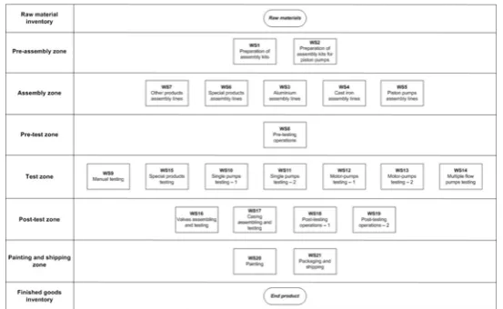
The workstations (WSs) of the assembling and testing area of the plant are reported and classified in Fig. 1. Note that the organization of Fig. 1 is mainly illustrative, because product routings are often not linear (i.e. not from top to bottom) and they seldom call at every zone of the assembling and testing area. For these reasons, as well as for the sake of comprehensibility, materials and information flow are not reported in Fig. 1.
The attention of the study was directed to the assembling and testing area because this is the core business of the firm itself. As Fig. 1 shows, this area can be divided into six zones between raw material inventory and finished goods inventory: (i) pre-assembling, (ii) assembling, (iii) pre-testing, (iv) testing, (v) post-testing, (vi) painting and shipping.
The pre-assembly zone (2 WSs) is the junction point between the inbound stock point and the
assembly zone: here the list of products to be manufactured is supplied by the MRP, and the workers, i.e. 4 people per shift on two 8-hour shifts a day, fill the assembly kits according to the Bill Of Materials.
The assembly zone (5 WSs) of the plant works on a single 8-hour shift and roughly assembles 2,600
products per day. The assembly operations vary according to the product variant; they can be carried out on a fixed-position assembly layout or an unpaced multi-model assembly line (for a classification of assembly lines see Scholl, 1999). This zone is directly fed by the pre-assembly zone and the assembly lines are divided as follows:
aluminium – 4 mixed-model unpaced assembly lines. Each line counts 3 assembly stations (i.e. 3 workers) that perform all of the assembly operations;
cast iron – 2 mixed-model unpaced assembly lines. Each line counts 3 assembly stations;
piston pumps – 3 fixed-position multi-model assembly lines. Each line counts 2 workers that pre-assemble products (if necessary) and carry out the entire assembly process;
special products – 6 fixed-position multi-model assembly lines. Each line counts 1 worker who pre-assembles products (if necessary) and carries out the entire assembly process;
other products – 1 fixed-position multi-model assembly line with 1 worker.
The main difference between the aluminium and the cast iron assembly lines is that the latter needs a subassembly operation for the mounting of bushings and bearings on the casing.
Within the pre-test zone (1 fixed-position multi-model assembly line with 1 worker), jobs coming
from the assembly zone may be modified and adapted to the following test zone. Examples of adjustments may be the assembling of multiple flow pumps, such as the cast iron-aluminium double pump or the piston-gear double pump. In order to assemble multiple pumps (i.e. WIP coming from different assembly lines), the synchronization of jobs is very important at this stage.
The test zone (7 WSs) is fed by the assembled products and processes every item; since product and
routing variability is very wide, the number of products entering the testing queue experience great variability too. The testing zone includes a total of 12 test benches: 2 benches each for WS10 to WS14,
and 1 bench for WS9 and WS15. The entire work cycle of the pump is performed at these benches and
burrs are created so as to ensure better operating conditions of the end product. As at the assembly zone, testing WSs and benches are classified according to the jobs they process. In this case, however, distinctions are not so important, since most of the benches may test most of the products (at the price of significantly longer setup times).
The test phase also verifies if the performances of the products comply with standards; if this should not be the case, the products are to undergo repairs and a new test is performed. The average defect rate is 2.5% and is not dependent on product family, batch, shift or raw materials (i.e. random). Since the testing zone processes more items than the assembly zone (because of repairs) and has long CTs (up to 45 minutes), it works on three 6.5-hour shifts per day.
The post-test zone operates on a single 8-hour shift per day, and counts 4 WSs with 1 worker each
In the painting and shipping zone (2 WSs) items are painted and prepared for shipping, when needed.
Before shipping, purchase orders must be fulfilled, i.e. all the items must be synchronized. This zone is directly fed by the post-test zone and works on a single 8-hour shift per day.
A close analysis of the firm suggests that the plant bottleneck is located at the test zone: indeed, these WSs appear to be the ones with the highest long term utilization (hence they work on three shifts per day), because of long CTs and the need to test every product at least once (or even twice, if repairs are needed).
3.2 Group jobs into families
The description hitherto presented has not mentioned CTs, SSDs and production rates of each workstation of the plant. All of these data, in fact, may be measured for each job at each WS, but there are far too many to manage. The number of different product codes, in fact, is roughly equal to 25,000, with an average process batch of 10 parts, while the workstations identified in this part of the plant amount to 21. For this reason, jobs were grouped into families with the same routing so as to allow the (future) simulation processes. The number of jobs was reduced from 25,000 different jobs to 195 different routings, each one passing in the same sequence through 21 WSs, though not necessarily through the same machine/assembly station at each WS.
3.3 Connect every family with an average value of CT and SSD
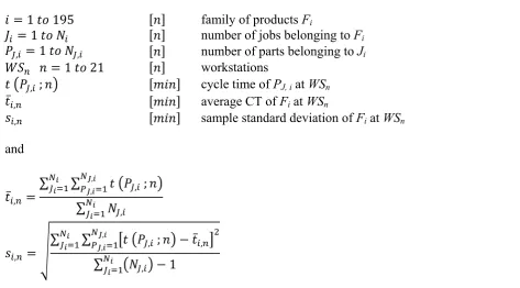
Each family of products was then associated with the total part number, average CT and SSD of all the product codes and part numbers belonging to it. The average CTs ( ̅, ) and SSDs ( , ) of every product family at each workstation were calculated as follows.
1 195 family of products Fi
1 number of jobs belonging to Fi
, 1 , number of parts belonging to Ji
1 21 workstations
, ; cycle time of PJ, i at WSn
̅, average CT of Fi at WSn
, sample standard deviation of Fi at WSn
and
̅, ∑ ∑ , ;
, ,
∑ , (1)
,
∑ ∑ , , ; ̅,
,
∑ , 1 (2)
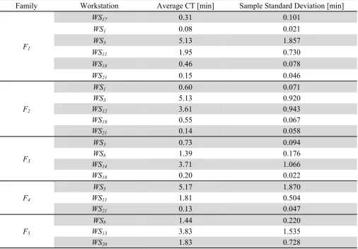
Table 2 reports the routing, ̅, and , for families from 1 to 5 according to Eq. (1) and Eq. (2) (see
also Bertolini & Romagnoli, 2013). For example, a part belonging to F3 will visit WS3 with an average
since values of CT and SSD are connected with families of different products (even if sharing the same routing), it may be that several products of a family experience simple operations at some WSs, and this leads to short average CTs;
it often happens that WS1 and WS21 experience simple operations (such as applying stickers or
preparing small kits) and this leads to short CTs at these WSs;
sometimes post testing operations only involve visual inspections on products;
finally, it may be seen that, though a dominant flow direction exists between WSs (i.e. ascending order), the workflow is not unidirectional (see for example F1).
Table 2
Average CTs and sample standard deviation for the first 5 families of products (Bertolini & Romagnoli, 2013)
Family
Workstation Average CT [min] Sample Standard Deviation [min]
F1
WS17 0.31 0.101
WS1 0.0210.08
WS3 5.13 1.857
WS11 0.7301.95
WS18 0.46 0.078
WS21 0.0460.15
F2
WS1 0.60 0.071
WS3 0.9205.13
WS12 3.61 0.943
WS18 0.0670.55
WS21 0.14 0.058
F3
WS3 0.73 0.094
WS8 0.1761.39
WS14 3.71 1.066
WS18 0.0220.20
F4
WS3 5.17 1.870
WS11 0.5041.81
WS21 0.13 0.047
F5
WS8 1.44 0.220
WS13 1.5353.83
WS20 1.83 0.728
3.4 Choose characteristics of the CONWIP system
After a close examination of the production system, we chose to simulate the implementation of a CONWIP production plan and control with multiple-product families and the following features (see Hopp & Spearman, 2008):
pull-from-the-bottleneck scheme: cards trigger strategy is based on the bottleneck status, where
the bottleneck was identified at the test zone, i.e. at WS9 to WS15. This means that cards only
flow from the beginning of each routing to the test zone, and the WIP level is held constant in the WSs up to and including the bottleneck;
path type cards: each card defines the WS in which testing will follow (i.e. the 7 testing WSs,
from WS9 to WS15), and therefore product families will be grouped according to their testing
traceability is higher, because we already know in which queue (in front of a testing workstation) the product will be waiting for processing; (iii) boxes (or posts) for CONWIP cards are smaller, though increased in number, and this improves internal logistics;
common unit to measure WIP: the sum of the working capacities (in minutes) that all the jobs
released will occupy at the 7 testing WSs.
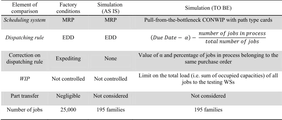
Current characteristics of the shop floor and assumptions made for the simulation of the present and future states of the system are summarized in Table 3.
Table 3
Assumptions and comparison between factory conditions and the present and future state simulations
Element of
comparison conditionsFactory Simulation (AS IS) Simulation (TO BE)
Scheduling system MRP MRP Pull-from-the-bottleneck CONWIP with path type cards
Dispatching rule
EDD EDD
Correction on
dispatching rule Expediting None Value of α and percentage of jobs in process belonging to the same purchase order
WIP
Not Not controlled controlled Limit on the total load (i.e. sum of occupied capacities) of all jobs to the testing WSs
Part transfer Negligible Not considered Not considered
Number of jobs
25,000 195 195 families families
3.5 Define the cards release strategy
The logic behind the releasing of the cards is illustrated below.
9 15 WS of the testing zone
1 number of jobs released that will be tested at WSn
maximum product load at WSn (working minutes)
residual capacity at WSn
, occupied capacity by job J at WSn
, 0; 1 releasing of a card for job J that will be tested at WSn
, 0; 1 finishing of job J at WSn
In this context, each one of the 7 testing WSs (let’s say WS11) will process a maximum number Mn of
jobs. In the same time, WS11 is characterized by a product load (L11), i.e. the process variable that
indicate the maximum total amount of WIP (expressed in testing minutes at station 11) allowed in the system for that specific working station, and by two variables, residual capacity (RC11) and the
capacity occupied by a general job J(OCJ, 11).
Each job J11 released in the system will occupy an average capacity of OCJ, 11 testing minutes at WS11,
and the residual capacity of a general WSn is defined in Eq. (3).
As Eq. (3) shows, RCn is always less than or equal to Ln. By means of RCn the system deals with the
possibility of releasing new cards for jobs that will be processed at WSn, as is shown below.
Initialization of the system
, 0
, 0
9 15
1
0 , 1 ; 1 ; ,
, 0
Running phase
, 1 ,
0 , 1 ; 1 ; ,
, 0
The first loop previously illustrated (initialization of the system) ends when all residual capacities are not positive, so no other card can be released in production. Afterwards, during the running phase, when the capacity of a general Jn is freed (for its test has finished), the OCJ, n is released and if RCn
becomes positive, the card for a new job to be tested at WSn will be released. In this way, we achieve a
CONWIP system capable of keeping WIP under control up to the bottleneck through path type cards by measuring WIP in minutes of occupied capacity at the testing workstation (WSn). Once released, jobs
follow their routing up to the testing zone: each time a job Jn finishes its test, the value of the occupied
capacity of Jn (OCJ, n) is added to the residual capacity of WSn (RCn), where n is the WS in which the
testing of Jn takes place. Fig. 2 shows a diagram of this process. As can be seen in Fig. 2, another main
difference between the current and the future state is the organization of the backlog list. By now, the backlog is a list of jobs to be processed sorted according to the EDD rule. In the future state, backlogs will be created for each testing WS, so as to create 7 different backlog lists associated with WS9 to
WS15. Section 3.6 explains how jobs will be released into the system from the backlog list, as well as
how they will be dispatched when queueing in front of a processing workstation.
3.6 Define a dispatching rule
According to the specific needs of the firm, the following goals were identified as guidelines for the scheduling problem:
punctuality on delivery of customer orders;
synchronization of customer orders (when belonging to the same purchase order);
priority to hot jobs.
W
Ac mi
Fig
e referred to
a = ma
b = pr
c = ob
Weigh
and 1 some p ccording to ix of:
EDD i
NUJO
purcha
applic days a
g. 2. cards r
o the Pinedo achine envir ocessing ch bjectives, w
hted Latenes
for normal
parts ‘wait’ Thiagaraja
in order to a
OB, modified ase order; cation of fac ahead of sch
release strat
o approach ronment, Fl
haracteristic which are (i)
ss of purch
l jobs, and because of an and Raje
apply a cont d so as to m
ctor α, whic hedule, whe
tegy, compa
(Pinedo, 20
lexible
Job-cs and const ) average jo hase orders.
the Staging f lack of syn endran (200
trol on item manage the
ch indicates n α > 0) so
arison betwe
002) a | b | c
-shop with 2
traints, Rele
ob Tardines
The weigh g Time is e nchronizatio 05), the disp
ms punctuali synchroniz
s the advan as to consid
een the curr
c, which ind 21 stages of
ease Time (r
s, (ii) avera ht criterion, equal to the on of purcha
patching ru
ity;
zation of dif
nce we plan der the impo
rent and the
dicates: f parallel ma
rj);
age Staging
w, is set eq wait-to-ma ase orders). ule for prod
fferent jobs
n to have (m ortance of a
e future state
achines (FJ
g Time and (
qual to 10 atch time (i
duct familie
belonging
measured in a hot order.
e
J21);
(iii) average for hot jobs i.e. the time
s shall be a
to the same
This leads to the following dispatching rule, where the fraction considers the ratio between the number of jobs already in process and the total number of jobs belonging to the same purchase order (see also Table 3):
: (4)
3.7 Build the simulation model of the current state
The simulation model that has been used is a discrete, dynamic and stochastic discrete-event simulation
model, implemented in an object-oriented software, Simul8 (release 12). The model of the assembling
and testing area has been organized in 21 workstations, with a variable number of parallel machines, and the simulation of each workstation was made with the utilization of ̅, and , , according to the product family (see Section 3.3). CTs and SSDs used in this model refer to year 2008. They are represented as normal distributions with , ~ ̅, ; , .
Replicating the conditions of the actual shop floor attentively, we created all the connections between job-shops and stock points, in order to simulate the routings of 195 product families Fi. For the
purposes of the simulation, Simul8 software was linked to several MS Excel worksheets, so as to allow the processing of a greater number of data (to the detriment of simulation times).
3.8 Validate the simulation model
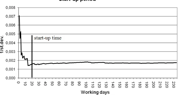
Particular attention was paid to the validation of the current state model. The steady state was graphically identified after a start-up period of 20 working days by monitoring the reciprocal of the standard deviation of daily production rate (see Fig. 3).
Fig. 3. start-up period definition
We then carried out 10 consecutive simulation runs of the current state, each lasting one year, and analysed their output, i.e. the average values of response variables.
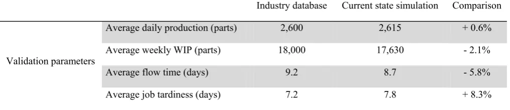
Table 4
Comparison between data from the firm’s database and the simulation (AS IS) for the validation of the model
Industry database Current state simulation Comparison
Validation parameters
Average daily production (parts) 2,600 2,615 + 0.6%
Average weekly WIP (parts) 18,000 - 17,630 2.1%
Average flow time (days) 9.2 8.7 - 5.8%
Average job tardiness (days) 7.2 + 7.8 8.3%
3.9 Build the simulation model of the future state
Once the validation of the current state was implemented, the future state model was built, in order to simulate a system with the characteristics described in Sections 3.4 to 3.6. Only two important process factors still need to be determined for the optimization of the future state, i.e. the maximum value of WIP allowed in the system and the value of α, the planned advance in due date for hot jobs (see Sections 3.4 and 3.5). Factors and levels at this step were chosen by mutual consent with the firm’s management, and they are reported in Table 5. We have proceeded with a quick Design Of Experiment (DOE) applied to the simulation process, according to Montgomery (2001).
Table 5
Factors and levels for the future state
Factors Lower Level (-) Higher Level (+)
A α - days ahead of schedule for important orders (days) 5 10
B 28,500WIP - sum of working minutes at testing WSs (minutes) 34,200
Table 6
Design matrix and results of the 22 factorial analysis
A B R1 R2 R3
Design
point α WIP
Average job Tardiness
Average Staging time
Average Weighted Lateness of purchase orders
(1) 28.5005 4,069,45 30,85
a 10 28.500 10,32 4,00 14,16
b 34.2005 4,009,06 19,20
ab 10 34.200 8,36 4,25 24,63
A1 = 0.09 A2 = 0.10 A3 = -5.63
B1 = -1.18 B2 = 0.10 B3 = -0.59
AB1 = -0.79
AB AB2 = 0.15 3 = 11.06
Response variables are reported in Section 3.6 (i.e. objectives of the a | b | c Pinedo approach). We applied a full factorial design and made a 22 sampling campaign with 10 replications. Replications were made by conducting “Trials” in the simulation software (i.e. a series of runs performed with all the same parameters in the simulation except for the random numbers). Results are displayed in Table 6, where each design point is characterized by a factor-level combination and an average outcome of the three response variables (R1; R2 and R3); at the same time, each response variable is related to the main
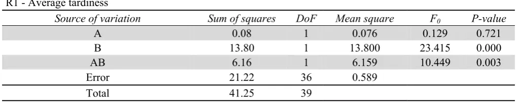
Table 7
ANOVA of the three response variables R1 - Average tardiness
Source of variation DoFSum of squares Mean square P-valueF0
A 0.08 1 0.076 0.129 0.721
B
13.80 13.8001 23.415 0.000
AB 6.16 1 6.159 10.449 0.003
Error
21.22 36 0.589
Total
41.25 39
R2 - Average staging time
Source of variation DoFSum of squares Mean square P-valueF0
A 0.09 1 0.091 0.491 0,488
B
0.09 0.0881 0.477 0.494
AB 0.25 1 0.251 1.357 0.252
Error
6.67 36 0.185
Total
7.10 39
R3 - Average weighted lateness
Source of variation DoFSum of squares Mean square P-valueF0
A 316.85 1 316.848 64.513 0.000
B
3.50 3.4981 0.712 0.404
AB 1,223.12 1 1,223.125 249.039 0.000
Error
176.81 36 4.911
Total
1,720.28 39
As it can be seen from Table 7, response variable number 2 (average staging time) is not influenced by any of the factors (minimum p-value is 0.252). However, factor B (WIP) significantly influences average job tardiness (R1), and factor A (alpha) influences average weighted lateness of purchase
orders (R3); furthermore, both R1 and R3 are influenced by the interaction between the factors (AB). If
we go back to Table 6, we can deduce that B1 (i.e. the main effect of B measured on R1) is negative but
small; that is an increase of B slightly diminishes average job lateness (which is good). On the other hand, A3 is negative but relatively big; and this means that an increase of A significantly diminishes
average weighted lateness of purchase orders. Furthermore, the interaction AB3 is positive and big, and
this means that, in order to limit R3, the factors must not be both at the high (or low) level (i.e. no ab
and no (1) combinations are recommended).
For these reasons, the best configuration was found to be design point a:
WIP = 28,500 minutes
α = 10 days
3.10 Simulate the future state
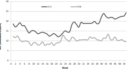
The results of the simulation and the comparison between the current and the future state of the system are reported in Fig. 4 and Table 8. Fig. 4 graphically shows the comparison in average WIP
(parts/week), while Table 8 reports average values and standard deviations in production, WIP, flow
Fig. 4. Comparison between WIP average levels (thousands of parts per week)
Table 8
Comparison between the current and the future state of the system
as is
to Comparisonbe
Production [parts/day] Average 2,615 2,561 -2.1%
Std Dev 18.712.7 +47.6%
WIP [parts/week] Average 17,630 10,238 -41.9%
Std Dev 325749 -56.6%
Flow time[days] Average 8.67 5.28 -39.1%
Std Dev 0.310.65 -52.3%
Job Tardiness [days] Average 7.80 10.32 +32.3%
Std Dev 0.66 0.63 -4.5%
Staging Times [days] Average 7.24 4.00 -44.8%
Std Dev 0.43 0.62 +44.2%
Weighted Lateness [days] Average 22.00 14.16 -35.6%
Std Dev 4.69 5.26 +12.2%
3.11 Analyse results
Let us consider the outcome of Fig. 4 and Table 8: the average level of WIP (parts/week) is greatly reduced in both its average value (- 41.9%) and its standard deviation (-56.6%); the same results could be achieved by measuring WIP in total working minutes at the testing zone, but this is quite obvious, since this parameter is directly controlled by the CONWIP system. Average flow times are also almost 40% shorter than before, and their standard deviation has decreased by more than 50%.
Tardiness (by more than 30%) without significantly modifying its standard deviation. This result is due to the importance given to hot jobs and to the synchronization of purchase orders. In fact, the application of the dispatching rule (Section 3.6) leads to significant reductions in average Staging Times and Weighted Lateness. In both cases, the increase in their standard deviations can be ascribed to the importance given to hot jobs.
Finally, the average daily production in the future state will be 2% smaller and its standard deviation will be increased, but these are relative losses. In fact, the current system is meeting demand, as often happens in MTO/ETO systems, and the demand profile is highly variable. At present, the plant experiences short order backlogs and high levels of WIP. However, as previously stated, the implementation of the simulated system will lead to lower weighted lateness and a considerable reduction of WIP (to the detriment of order backlogs). Potential consequences of these differences should be gain in market shares, economic savings and, finally, the possibility to invest in new test benches, thus increase bottleneck capacity and productivity.
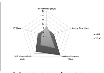
A visual comparison of results is reported in Fig. 5. We can therefore conclude that the system we have simulated (future state) has fulfilled 2 objectives (out of the three defined) with a significant reduction in flow times and WIP and without significantly affecting the production rate.
Unfortunately, the firm has so far not proceeded with the implementation of the future state, so Section 3.12 is not reported.
Fig. 5. comparison of average results on a radar diagram
4. Conclusions
The results we have achieved confirm the validity of CONWIP. Average WIP, measured in parts per week, decreased by over 40% and its standard deviation by over 50% without significantly affecting production rate; flow times were also reduced in both their average values and their standard deviation. The reduction in WIP and flow time standard deviations is extremely important, because it can ensure more precise and robust values to rely on when planning production. The dispatching rule we have chosen was evaluated using three indicators that express the system’s capacity to meet management requirements. These indicators are (i) average tardiness, measuring order punctuality, (ii) average staging time, indicating the synchronization of parts belonging to the same purchase order, and (iii) average weighted lateness, reporting the ability to ensure punctuality of hot jobs. All of these indicators were measured in 10 simulation runs and reported in their average values and standard deviations. The synchronization of purchase orders was considerably increased, by reducing average staging time to 4 days (- 44%), and average weighted lateness was decreased by 36%, that is greater attention was paid to hot jobs. Nevertheless, these achievements led to the growth (+ 32%) of average job tardiness, though this result was partially expected: one of the goals of the dispatching rule we adopted is to increase the priority of hot jobs, to the detriment of normal ones and with the increase in average (non-weighted) tardiness. For all of these reasons, we can state that the proposed solution could be an excellent scheduling and control system for the shop floor of a complex manufacturing firm, being integrated in a planning system such as (classic) MRP.
Possible future developments of this study may be the optimization of model factors in a systematic way (i.e. not only relying on practical experience of the firm’s management and common sense). On the other hand, especially when dealing with everyday scheduling problems of the SF, an on-line simulation may be the only way to achieve optimum results in a reasonable amount of time.
Finally, it is important to remark that the main drawback in this approach, even though it is applied to a real manufacturing environment, lies in the impossibility of providing optimum results without the comparison and evaluation of a certain number of different planning and control systems (such as synchro-MRP, workload control and drum-buffer-rope) and/or dispatching rules.
References
Adetunji, O.A.B. & Yadavalli, S.V. (2012). An integrated utilisation, scheduling and lot-sizing algorithm for pull production, International Journal of Industrial Engineering: Theory, Applications
and Practice, 19(3).
Anavi-Isakow, S. & Golany, B. (2003). Managing multi-project environments through constant work-in-process, International Journal of Project Management, 21(1), 9-18.
Benton, W.C. & Shin, H. (1998). Manufacturing Planning and Control: The evolution of MRP and JIT integration, European Journal Of Operational Research, 110(3), 411-440.
Bertolini, M., Braglia, M., Romagnoli, G. & Zammori, F. (2013). Extending value stream mapping: the synchro-MRP case, International Journal of Production Research, 51(18), 5499-5519.
Bertolini, M. & Romagnoli, G. (2013). Design and simulation of multi-CONWIP into a Make-To-Order firm with General Job Shop configuration, Proceedings of the 43rd International Conference on Computers and Industrial Engineering (CIE43), 16-18 October 2013, Hong Kong, China.
Bonvik, A.M., Couch, C.E. & Gershwin, S.B. (1997). A comparison of production-line control mechanisms, International Journal of Production Research, 35(3), 789-804.
Braglia, M., Frosolini, M., Gabbrielli, R. & Zammori, F. (2011). CONWIP card setting in a flow-shop system with a batch production machine, International Journal of Industrial Engineering
Computations, 2(1), 1-18.
Chong, M.Y., Prakash, J., Ng, S.L., Ramli, R. & Chin, J.F. (2013). Parallel Kanban-ConWIP system for batch production in electronics assembly, International Journal of Industrial Engineering:
Duri, C., Frein, Y. & Lee, H.-S. (2000). Performance evaluation and design of a CONWIP system with inspections, International Journal of Production Economics, 64(1), 219-229.
Enns, S.T. (1995). An economic approach to job shop performance analysis, International Journal of
Production Economics, 38(2-3), 117-131.
Flapper, S.D.P., Miltenburg, G.J. & Wijugard, J. (1991). Embedding JIT into MRP, International
Journal of Production Research, 29(2), 329-341.
Framinan, J.M., González, P.L. & Ruiz-Usano, R. (2003). The CONWIP production control system: review and research issues, Production Planning & Control, 14(3), 255-265.
Framinan, J.M., González, P.L. & Ruiz-Usano, R. (2006). Dynamic card controlling in a CONWIP system, International Journal of Production Economics, 99(1-2), 102-116.
Geraghty, J. & Heavey, C. (2004). A comparison of Hybrid Push/Pull and CONWIP/Pull production inventory control policies, International Journal of Production Economics, 91(1), 75-90.
Gibson, P., Greenhalgh, G. & Kerr, R. (1995). Manufacturing Management: Principles and concepts,
London: Chapman & Hall.
Hall, R.W., (1981). Driving the productivity machine: Production planning and control in Japan, Falls Church, Virginia: American Production and Inventory Control Society.
Hodgson, T.J. & Wang, D. (1991). Optimal hybrid push/pull control strategies for a parallel multistage system: Part I, International Journal of Production Research, 29(6), 1279-1287.
Hopp, W.J. & Spearman, M.L. (2008). Factory Physics, 3rd ed., Dubuque, Iowa: McGraw-Hill/Irwin. Huang, M., Wang, D. & Ip, W.H. (1998). Simulation study of CONWIP for a cold rolling plant,
International Journal of Production Economics, 54(3), 257-266.
Koulouriotis, D.E., Xanthopuolos, A.S. & Tourassis V.D. (2010). Simulation optimisation of pull control policies for serial manufacturing lines and assembly manufacturing systems using genetic algorithms, International Journal of Production Research, 48(10), 2887-2912.
Lambrecht, M.R. & Decaluwe, L. (1988). JIT and constraint theory: the issue of bottleneck management, Production and Inventory Management Journal, 29(3), 61-65.
Larsen, N.E. & Alting, L. (1993). Criteria for selecting a production control philosophy, Production
Planning and Control, 4(1), 54-68.
Lengyel, A., Hatono, I. & Ueda, K. (2003). Scheduling for on-time completion in job-shops using feasibility function, Computers & Industrial Engineering, 45(1), 215-229.
Li, G.-W. (2010). Simulation study of coordinating layout change and quality improvement for adapting job shop manufacturing to CONWIP control, International Journal of Production
Research, 48(3), 879-900.
Mahdavi, I., Shirazi, B. & Solimanpur, M. (2010). Development of a simulation-based decision support system for controlling stochastic flexible job shop manufacturing systems, Simulation Modelling
Practice and Theory, 18(6), 768-786.
Monden, Y. (1998). Toyota Production System, An Integrated Approach to Just-In-Time, 3rd ed., Norcross, Georgia: Chapman & Hall.
Montgomery, D.C. (2001). Design and analysis of experiments, 5th ed., New York, New York: John Wiley & Sons.
Ohno, T. (1988). Toyota Production System: Beyond Large-Scale Production, New York, New York: Productivity Press.
Özbayrak, M., Papadopoulou, T.C. & Samaras, E. (2006). A flexible and adaptable planning and control system for an MTO supply chain system, Robotics and Computer-Integrated Manufacturing, 22(5-6), 557-565.
Pettersen, J.A. & Segerstedt, A. (2009). Restricted work-in-process: A study of differences between Kanban and CONWIP, International Journal of Production Economics, 118(1), 199-207.
Pinedo, M. (2002). Scheduling: theory, algorithms and systems, 2nd ed., Upper Saddle River, New Jersey: Prentice Hall.
Renna, P. (2010). Dynamic control card in a production system controlled by CONWIP approach,
Jordan Journal of Mechanical and Industrial Engineering, 4(4), 425-432.
Roderick, L.M., Toland, J. & Rodriguez, F.P. (1994). A simulation study of CONWIP versus MRP at Westinghouse, Computer & Industrial Engineering, 26(2), 237-242.
Rubiano Ovalle, O. & Crespo Marquez, A. (2003). Exploring the utilization of a CONWIP system for supply chain management. A comparison with fully integrated supply chains. International Journal
of Production Economics, 83(2), 195-215.
Scholl, A. (1999). Balancing and sequencing of assembly lines, 2nd ed., Munich: Physica Verlag.
Sharma, S. & Agrawal, N. (2009). Selection of a pull production control policy under different demand situations for a manufacturing system by AHP-algorithm, Computer & Operations Research, 36(5), 1622-1632.
Spearman, M. L., Woodruff, D. L. & Hopp, W. J. (1990). CONWIP: a pull alternative to kanban,
International Journal Of Production Research, 28(5), 879-894.
Stevenson, M., Hendry, L.C. & Kingsman, B.G. (2005). A review of production planning and control: the applicability of key concepts to the make-to-order industry, International Journal of Production
Research, 43(5), 869-898.
Sultana, I & Ahmed, I. (2014). A state of art review on optimization techniques in just in time.
Uncertain Supply Chain Management, 2(1), 15-26.
Thiagarajan, S. & Rajendran, C. (2005). Scheduling in dynamic assembly job-shops to minimize the sum of weighted earliness, weighted tardiness and weighted flowtime of jobs, Computers &
Industrial Engineering, 49(4), 463-503.
Villa, A. & Watanabe, T. (1993). Production management: beyond the dichotomy between push and pull, Computer Integrated Manufacturing Systems, 6(1), 53-63.
Vollmann, T.E., Berry, W.L. & Whybarck, D.C. (1997). Manufacturing planning and control systems, 4th ed., New York, New York: McGraw-Hill.
Yang, T., Fu, H.P. & Yang, K.Y. (2007). An evolutionary-simulation approach for the optimization of multi-constant work-in-process strategy – A case study, International Journal of Production