VOLUME 37, ARTICLE 12, PAGES 325
,
362
PUBLISHED 15 AUGUST 2017
http://www.demographic-research.org/Volumes/Vol37/12/ DOI: 10.4054/DemRes.2017.37.12
Research Article
Childlessness and fertility by couples’
educational (in)equality in Austria, Bulgaria,
and France
Beata Osiewalska
© 2017 Beata Osiewalska.
This open-access work is published under the terms of the Creative Commons Attribution NonCommercial License 2.0 Germany, which permits use, reproduction, and distribution in any medium for noncommercial purposes, provided the original author(s) and source are given credit.
1 Introduction 326
2 Research hypotheses 328
3 Methodology 333
3.1 Data and covariates 333
3.2 Hurdle zero-truncated Poisson model with Bayesian approach 337
4 Results and discussion 339
5 Robustness checks 347
5.1 Measures of education 347
5.2 Model comparison 349
5.3 Control covariates 349
6 Conclusions 350
7 Acknowledgements 351
References 352
Childlessness and fertility by couples’ educational (in)equality
in Austria, Bulgaria, and France
Beata Osiewalska1
Abstract
BACKGROUND
In modern, highly developed countries the association between education and fertility seems to be equivocal: A negative influence of education mainly applies to women, while among men the correlation is often positive or negligible. Although the gender differences have been examined in depth, couples’ procreative behaviour treated as the result of a conflict between male and female characteristics is still understudied.
OBJECTIVE
This study aims to investigate couples’ reproductive behaviour among contemporary European populations with regard to (in)equality between partners’ educational levels and the joint educational resources of a couple. Various measures of educational endogamy are considered.
METHODS
The hurdle zero-truncated Poisson model within the Bayesian framework is applied. The data comes from the first wave of the Generations and Gender Survey for Austria, Bulgaria, and France.
RESULTS
Homogamous low-educated partners have, on average, the highest fertility. The highly educated postpone childbearing and have a smaller number of children in all countries except France, where their completed fertility does not differ from that of other unions. The effect of hypergamy is insignificant and is thus similar to homogamy in medium education. Hypogamy negatively influences fertility in Bulgaria and Austria, while in France the effect is insignificant.
CONCLUSIONS
The small variation in fertility due to couple-level education observed in France indicates that proper institutional support for families might help couples overcome possible obstacles and enhance fertility for all educational profiles.
CONTRIBUTION
This study provides a perspective on the relationship between reproductive behaviour and educational pairing in varying country-specific contexts. It reaches key conclusions on contemporary fertility regarding both childlessness and parenthood and their association with couples’ different educational profiles.
1. Introduction
Much research, as mentioned above, deals with the problem of determining the association between educational level and fertility, but most of it concentrates on only women or only men. What the literature to date lacks is a complex analysis of fertility from a couple perspective. Some studies have examined the influence of both partners’ individual education on their mutual fertility decision-making process (Bauer and Kneip 2013) and fertility behaviour (Gerster et al. 2007 on Denmark, Vignoli, Drefahl, and De Santis 2012 on Italy, Begall 2013 on the Netherlands, Begall and Mills 2013 on the Netherlands, Jalovaara and Miettinen 2013 on Finland). A few studies focus on the couple as a unit and consider the combined educational levels of the partners (Bauer and Jacob 2009 on Germany, Osiewalska 2015 on Poland). This couple approach is important because in modern societies fertility decisions are not taken solely by men or women but are the result of mutual preferences and compromises between both potential parents, taking into account the individual opportunity costs of both sides (Begall 2013; Doepke and Kindermann 2016). Since fertility decisions are made by a couple, each partner considers not only his or her own desires and prospects but also the resources and plans of the other partner. When considering having a child, a highly educated woman whose partner is also highly educated might come to a very different decision than if her partner were low-educated. Thus, rather than the partners’ individual characteristics, the relative socioeconomic characteristics could have an even greater impact on reproductive behaviour (Bauer and Jacob 2009).
The aim of this study is to investigate reproductive behaviour in contemporary European populations with regard to a couple’s educational resources. In particular, it aims to determine whether educational gender equality or inequality within a couple influences the risk of childlessness and the mean number of children. The possible impact of the level of a couple’s joint resources is also examined. The populations of childless partners and of parents are linked within a single model by the probability of childlessness/parenthood. Besides educational level, the following socioeconomic characteristics of a couple and their household are considered and included in the model as control variables: total household income, number of hours worked per week, and institutional help with childcare.
highly educated individuals (Wood, Neels, and Kil 2014; Winkler-Dworak and Toulemon 2007). In Bulgaria the educational gradient in childlessness is generally positive but is much weaker than in Austria and France (Wood, Neels, and Kil 2014; Sobotka 2015). The between-country variation in the relationship between education and fertility indicates its sensitivity to context (e.g., the availability of childcare, women’s societal position, the level of gender equality), which is especially prominent among highly educated individuals. The country-specific context of reproductive decisions is complemented by the micro-level couple profile. Considering couple-level education may shed more light on how reproductive behaviour is shaped, in view of different joint resources or educational (in)equality between partners. Taking the country-comparative perspective may reveal how the fertility of couples with varying educational profiles is differentiated by contextual factors.
The next section discusses hypotheses formulated on the basis of the theoretical background and previous findings. Section 3 describes the data used in the study together with the set of covariates and a brief description of the methodology. Section 4 presents the estimations of the models’ parameters and comments on the results. Section 5 demonstrates the robustness of the results with regard to different measures of educational endogamy and control covariates. Finally, Section 6 presents the general conclusions.
2. Research hypotheses
2000). Traditional gender roles assign household tasks to women and the supply of resources to men. While such specialisations might be beneficial in hypergamous partnerships in which the man is more educated than the woman, in hypogamous unions the traditional allocation of duties might impose a double burden on the better-educated female partner, who can end up being responsible for both providing economic resources and doing the household tasks. When partners’ specialisations are thus unequal, couples’ reproduction is often postponed and limited (Oppenheimer 1994; Matysiak and Vignoli 2008). To increase the level of fertility in developed societies an increase in gender equality is required (Anderson and Kohler 2015; Esping-Andersen and Billari 2015; Goldscheider, Bernhardt, and Lappegård 2015). More flexible gender roles allow couples to adjust their specialisations to prevailing family conditions, and in particular for males and females to both participate in housework and childcare.
The three selected countries – Austria, Bulgaria, and France – provide different contexts and distinct conditions for fertility analysis. The level of fertility is relatively low in Austria and Bulgaria compared to other European countries, while France has one of the highest levels of fertility in Europe. In Bulgaria, our representative of postsocialist countries, high female labour force participation was the norm much earlier than in Western Europe, and the cultural change from the traditional male-breadwinner family model to the two-male-breadwinner model happened earlier than in Austria or France. Meanwhile, the attitudes towards gender roles in housework and childcare were traditional, and men remain resistant to domestic work. The level of gender equality in household duties has been much lower in Austria and France since the 1960s than in Scandinavia, but much higher than in Southern or Eastern Europe (Kan, Sullivan, and Gershuny 2011; Lesthaeghe and Permanyer 2014). Austria’s framework for work–family balance is far from perfect, as is reflected in its childcare system. Austria has a conservative welfare state, and its family policy is based on the traditional assumption that the family is responsible for childcare (Esping-Andersen 1990; Anttonen and Sipilä 1996). Thus, there are not enough facilities for young children, while for older children school hours are inadequate, ending early, and there is poor afterschool supervision (Lesthaeghe and Permanyer 2014). As a result there is low participation in childcare and preschool services (OECD 2016). In Bulgaria under state socialism, family policy was adjusted to the high participation of women in the labour force, and the availability of public childcare for working mothers was relatively high (Frejka 2008). After the collapse of the socialist regime the family policy was modified and the availability of public childcare declined. This turned out to be mismatched to the changing economic reality, and nowadays Bulgaria has an unadjusted childcare system, insufficient childcare facilities, and one of the lowest childcare participation rates in Europe (OECD 2016). In France, the childcare system is much better than in the other countries considered here. The availability of childcare is sufficient, and consequently the participation rate in formal childcare and other preschool services is high (OECD 2016); France has one of the most efficient childcare systems in Europe. Finally, Bulgaria differs from the other countries with regard to labour market conditions. Since the collapse of the state socialist system, job stability has significantly declined and the labour market has become competitive and harsh, resulting in high total unemployment and high youth unemployment (Frejka 2008). In addition, female labour force participation has declined and is now below the levels observed in Austria and France.
In countries with an inadequate childcare system, couples’ overall educational status influences their fertility so that homogamous highly educated partners have limited and postponed reproduction and homogamous low-educated couples have enhanced fertility
(H1).
This expectation is based on the high opportunity costs of childbearing for highly educated partners, which are especially salient in the context of a poor childcare system. Therefore, this hypothesis is expected to apply to Austria and Bulgaria. However, in the latter country this correlation is mainly associated with the effect of female education, since men, in a situation of asymmetric and traditionally apportioned domestic work, experience much smaller childbearing costs, regardless of their educational level. It is also anticipated that:
In Bulgaria, low-educated partners, because of general economic insecurity (low resources in addition to a high unemployment rate and lack of childcare) postpone childbearing and limit their number of children, compared to their highly educated counterparts (H1a).
This hypothesis might apply particularly to young couples that started their reproductive careers after the collapse of the state socialism. Finally, in France, because of well-adjusted childcare and schooling organisation, the opportunity cost of having a child might be lower than in the other countries analysed here. Women are often supported by their partners in household duties (Kan, Sullivan, and Gershuny 2011) and obtain adequate institutional help with childcare (Neyer 2003). In such cases, as suggested by Liefbroer and Corijn (1999), the effect of education on completed fertility might be weaker. Thus:
In France we expect only a small variation in the completed number of children according to couples’ educational status. However, among tertiary-educated partners, due to prolonged engagement in education and the importance assigned to professional development, we anticipate the occurrence of the postponement effect, especially regarding entry into parenthood(H1b).
Secondly, hypogamy in education (higher female than male education) is expected to have a negative impact on the tempo and quantum of fertility in Austria and Bulgaria. Thus:
The explanation for the negative effect of hypogamy on fertility is the lower level of support provided by the man to maintain his family (as the lower-educated partner usually provides a lower income) and the poor childcare system. Having a child is related to a temporary break in female labour marker participation and a potential decrease in income, both of which may create financial insecurity, especially if adequate childcare has to be paid for. Additionally, the job instability, high unemployment, and gender imbalance in household duties present in Bulgaria entail a high opportunity cost of childbearing, which mainly concerns females. As a consequence, the decision to have a child might be postponed or abandoned. In turn, the situation in France (good childcare, higher gender equality) might help hypogamous unions to overcome possible obstacles, and thus we claim that:
In France there is no significant difference between the tempo and quantum of fertility of hypogamous and hypergamous unions(H2b).
This expectation is supported by the study of Winkler-Dworak and Toulemon (2007), which shows that the gender-specific impact of educational level on fertility in France has converged over time so that the effect of male and female education on reproductive behaviour has become similar.
Finally, we expect that:
Hypergamy (higher male than female education) has a positive influence on reproductive behaviour, regarding both the tempo of childbearing and the number of children (H3).
3. Methodology
3.1 Data and covariates
The first waves of Generations and Gender Survey (GGS) data for Austria (year 2008‒ 2009), Bulgaria (2004), and France (2005) are used in this study (Generation and Gender Programme 2015,www.ggp-i.org). Only respondents who are in a coresidential relationship and are aged 24 or older in the original dataset are included in the final sample. Younger respondents, because of the high probability of yet unfinished educational careers, are not considered. Additionally, the sample only consists of couples in which the female partners are aged 45 or less.2 Those who cannot have
children for biological reasons (less than 1% of the initial sample size in each country) or who have children from different partnerships (14% of the initial sample size in Austria and France, 5% in Bulgaria) are not analysed. The final sample consists of 2,370 couples in Austria, 2,922 in Bulgaria, and 2,147 in France. Two important data limitations must be taken into account. The first one is the selection effect caused by the couple perspective. Due to insufficient information about partnership history, only respondents in a relationship at the time of interview were analysed. Single parents and the widowed or divorced were not included. In order to keep the sample homogeneous according to fertility behaviour, respondents in a relationship but with children from previous partnerships were not included. The second limitation is connected to analysing females of reproductive age, which implies that fertility might not be completed; we can study the number of children ever born but not the complete fertility of a couple. Therefore, this analysis might contain both tempo and quantum effects (compare Baudin 2015). For instance, higher-educated individuals might have a higher probability of having no children, which could be caused either by postponing the first childbirth or by the higher chance of definite childlessness. Similarly, having a low number of children could be explained either by the postponement of higher-order births or by the choice to have a smaller family size. To help distinguish tempo and quantum effects, the impact of education on fertility will be examined by female partners’ age.
The response variable in this study is the number of children ever born. The structure of this variable among couples with female partners aged 24‒45 is presented in Figure 1. In all the analysed countries, having two children is the most typical family model. The biggest share of childless couples is observed in Austria (19%), while it is
2 The Austrian GGS includes only respondents between 18 and 45 years old, while in Bulgaria and France
slightly lower in France (15%) and much lower in Bulgaria (5%). In Bulgaria there are very few couples with more than two children (only 6%), while in France and Austria larger families are more common (21% and 18% respectively).
Figure 1: Structure of number of children ever born, by country
Source: Author’s own elaboration based on the GGS sample.
The main explanatory variable considered in this analysis is the couples’ educational status. The variable is based on the combination of partners’ individual education levels, which in the GGS database are classified according to the ISCED-97 (from 0 for preprimary to 6 for the second stage of tertiary education).3 For the purpose
of this analysis, education is grouped into five classes (Measure 1):
∂ edu11 – both partners have at most low education (ISCED codes 0 through 2)
∂ edu22 – both partners have a medium educational level (ISCED codes 3 and 4; reference level)
∂ edu33 – both partners have completed a high level of education (ISCED codes 5 and 6)
∂ eduLH – hypergamous union: the woman has a lower educational level than the man in the couple, whether, respectively for the woman and the man, low– medium education, low–high education, or medium–high education
∂ eduHL –hypogamous union – the woman is more highly educated than the man, whether, respectively for the woman and the man, medium–low education, high–low education, or high–medium education.
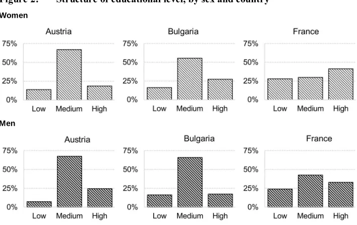
The structure of the analysed sample by education and sex in all the considered countries is presented in Figure 2. In Bulgaria and France the gender gap in education is
3 ISCED-97 – International Standard Classification for Education introduced by UNESCO in 1997. For
reversed: There are more highly educated women than men, while the opposite holds for Austria. In France there is little variation in educational level for both sexes.
Figure 2: Structure of educational level, by sex and country
Women
Men
Source: Author’s own elaboration based on the GGS sample
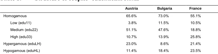
Table 1: Structure of couples’ educational status
Austria Bulgaria France
Homogamous 65.6% 73.0% 55.1%
Low (edu11) 3.8% 11.5% 10.5%
Medium (edu22) 51.1% 47.6% 18.8%
High (edu33) 10.7% 13.9% 25.8%
Hypergamous (eduLH) 23.0% 8.6% 21.4%
Hypogamous (eduHL) 11.4% 18.4% 23.5%
Source: Author’s own elaboration based on the GGS sample
Three groups of control covariates are considered in the analysis. The first group is the household’s socioeconomic characteristics. These are:
∂ household monthly income (low, medium [ref.], high)4
∂ number of hours worked per week by the woman (none, 20 or fewer, 21 to 40 [ref.], 41 or more)
∂ number of rooms in the flat/house (included as a number)
∂ whether the woman is a housewife (dummy).
It is important to underline that while education can be treated as completed before starting a family and, once obtained, not subject to depreciation, the other socioeconomic characteristics are subject to change. What is more, the causality between number of children and income, number of hours worked per week, or being a housewife might act in both directions: The second could determine the first (e.g., higher income could encourage women to have more children), but also the first could influence the second (a bigger family might create pressure to earn a higher income). Causality is difficult to capture using GGS cross-sectional data, which is why in this study we are able to measure the association of socioeconomic control characteristics with fertility but cannot identify the causality. The robustness of the results due to the inclusion or exclusion of these control variables will be examined.
The second group of control covariates comprises the following couple characteristics: marital status (married [ref.], cohabiting), age of the woman and man
4 For Austria and France: low HH income = less than 2,500 EUR per month; medium HH income =
(both standardised with a mean of 30 years old), and type of settlement (urban [ref.], rural), as well as all significant interactions between the age of the woman and the educational status of the couple. The interactions are considered in order to determine whether the effect of education on reproductive behaviour changes with the age of an individual, which in particular might help to distinguish tempo and quantum effects.
Finally, the third group consists of one covariate that is only included for parents: institutional help with childcare (whether a couple uses the institutional childcare system). This covariate may also be endogenous, as it is an indicator of the presence of young children in the family. The possible changes in the results, once adjusted for this variable, will be examined.
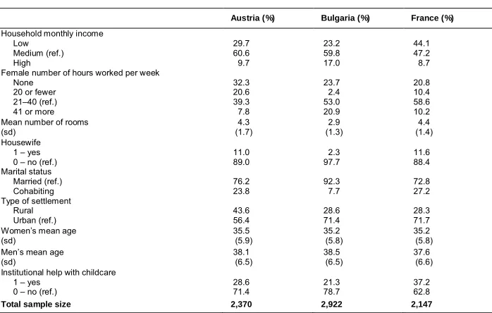
The structure of all control covariates is presented in Table 2.
Table 2: Structure of control variables
Austria (%) Bulgaria (%) France (%) Household monthly income
Low Medium (ref.) High 29.7 60.6 9.7 23.2 59.8 17.0 44.1 47.2 8.7 Female number of hours worked per week
None 20 or fewer 21‒40 (ref.) 41 or more
32.3 20.6 39.3 7.8 23.7 2.4 53.0 20.9 20.8 10.4 58.6 10.2 Mean number of rooms
(sd) 4.3 (1.7) 2.9 (1.3) 4.4 (1.4) Housewife
1 – yes 0 – no (ref.)
11.0 89.0 2.3 97.7 11.6 88.4 Marital status Married (ref.) Cohabiting 76.2 23.8 92.3 7.7 72.8 27.2 Type of settlement
Rural
Urban (ref.) 43.656.4 28.671.4 28.371.7
Women’s mean age
(sd) 35.5(5.9) 35.2(5.8) 35.2(5.8)
Men’s mean age (sd) 38.1 (6.5) 38.5 (6.5) 37.6 (6.6) Institutional help with childcare
1 – yes
0 – no (ref.) 28.671.4 21.378.7 37.262.8
Total sample size 2,370 2,922 2,147
Source: Author’s own elaboration based on the GGS sample.
3.2 Hurdle zero-truncated Poisson model with Bayesian approach
Poisson Model (HPM) (Pohlmeier and Ulrich 1995; Cameron and Trivedi 1998; Long and Freese 2006). Two different states, driven by different processes, are distinguished in the model. The first one, the zero state, is generated by a binary process and occurs with the probabilityp; in fertility this part stands for childlessness andp corresponds to the probability of being childless. The second one, the count state, takes positive integer values and is generated by the standard Poisson model truncated at zero. Thus, the basic idea behind the model is to join two different statistical distributions: the Poisson and the binomial. The binomial part governs the binary outcome and indicates whether the count variable has a zero (with probabilityp) or a positive realisation (with probability 1-p). If a threshold (‘hurdle’) is crossed, the variable takes a positive realisation and the Poisson part drives the probability. The formula for the model is written as follows:
⊆ < , , , , < < < ]. 1 , 0 [ ,..., 2 , 1 , ! ) exp( ) exp( 1 1 0 , ) , | ( i i i i y i i i i i i i i p y y p y p y Y P κ κ κ χ φ (1)
The regressions for zero and count states can be written as follows:
where
x
i andw
i are vectors of covariates for thei-th observation, and φ and χ are vectors of hyperparameters.In fertility modelling it is important that the specification of the model allows childlessness to be treated as a qualitatively different state from having children. The hurdle specification of the model distinguishes separate processes that drive zero (childlessness) and positive counts (parenthood). In order to include different determinants for childlessness and for parenthood, both parts are modelled separately, but at the same time both are connected to each other by applying the probabilityp. Moreover, the hurdle specification is flexible and is able to describe too many or too few zeros occurring in the sample; thus, for this analysis the model is necessary in order to explain the very different levels of childlessness observed in the analysed countries.
In this study Bayesian methods are used, with the prior distributions for the model’s hyperparameters [ ] and [ ] assumed to be multivariate normal distributions: ~ 0[ ]; [ ] and ~ 0[ ]; 0.05 [ ] . Bayesian
methods have recently become more popular in demography, especially in the area of population projection (Raftery et al. 2012; Bryant and Graham 2013; Wiśniowski et al. 2015) and migration (e.g., Bijak 2011; Abel et al. 2013). In fertility studies these
, ,..., 1 ),
exp(wi i n
i < χ <
methods have been used in forecasting (Schmertmann et al. 2014) and modelling (Osiewalska 2015, 2013). Bijak and Bryant (2016) recently carried out an overview of the use of Bayesian methods in demography.
4. Results and discussion
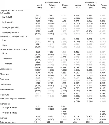
The effects of the different types of couples’ educational status on the probability of being childless and the risk of having subsequent children are summarised by the a posteriori distributions of the coefficients included in the analysis. The expected values of the coefficients and the corresponding measures of the variables’ significance are presented in Table 3. The presented measure of a variable’s significance (MS) is the marginal a posteriori probability that the parameter is equal to zero, which, for a given parameter πi, can be written as P(πi;0|Y) when E(πi|Y)″0, or P(πi=0|Y) otherwise. In this study we assume that values lower than 0.05 indicate a significant impact of the corresponding covariate on the response variable. Otherwise, when the MS exceeds a level of 0.05, a high probability that the parameter is equal to zero is reported, and the corresponding covariate is assumed to be negligible. When the variable is insignificant the values in Table 3 have been marked in grey.
Interpretations of the a posteriori expected values of the coefficients, presented in Table 3, are as follows. In the zero part of the model (childlessness), the probability of zero (probability of childlessness) is the main interest. The positive expected value of the coefficient indicates a higher probability of childlessness. The coefficients are interpreted in a similar way to those in the logistic model: The odds of being childless change by a factor exp (expected value of coefficients) for a unit increase in the corresponding covariate. The count part of the model is driven by the mean of the Poisson distribution (λ) and represents parenthood. The a posteriori expected values of the coefficients within this state are interpreted as in the standard Poisson regression model: Parents’ average expected number of children (represented by λ) changes by a factor exp (expected value of coefficient) for a unit increase in the corresponding covariate.
have a smaller family/not have children at all. In France, the interactions between the age of the woman and homogamy in high education suggest that it might be the effect of postponement rather than the quantum effect in fertility, since the probability of childlessness decreases and the average number of children increases as women get older.5 This interaction was found to be insignificant in Austria and Bulgaria, thus
implying that reduced completed fertility might be taking place in these countries. The impact of other educational statuses differs by country. Homogamous low-educated partners have a lower probability of being childless than medium-low-educated unions, but this effect is only significant in Austria and Bulgaria, where the chance of partners with a low level of education being childless is just a quarter of that of medium-educated couples (odds ratio of 0.23). Furthermore, in these two countries low-educated partners have a higher number of children than their counterparts. Thus, the effect of joint educational resources on couples’ reproductive behaviour was found to be negative in all the considered countries (hypothesis H1 confirmed, H1a rejected). In France, however, this negative effect only concerns partners with high educational levels and might be linked to the postponement of childbearing (hypothesis H1b confirmed). What is more, the significant interaction between the woman’s age and homogamy in low education suggests that the risk of childlessness for homogamous low-educated couples increases for older women in all the considered countries.
5 Although the probability that the coefficient standing for the interaction between a woman’s age and
Table 3: A posteriori expected values of coefficients and measures of significance (MS) in zero-state (childlessness) and count-state (parenthood) regressions
Childlessness (p) Parenthood (λ) Austria
(MS)
Bulgaria (MS)
France (MS)
Austria (MS)
Bulgaria (MS)
France (MS) Couples’ educational status
(ref. edu22)
low (edu11) ‒1.413 ‒1.489 0.031 0.404 0.457 0.096
(0.013) (0.005) (0.465) (0.001) (0.000) (0.101)
high (edu33) 0.855 0.568 1.018 ‒0.174 ‒0.160 ‒0.298
(0.002) (0.032) (0.001) (0.036) (0.034) (0.006)
hypergamy (eduLH) 0.085 ‒0.387 0.057 0.051 0.057 ‒0.020
(0.349) (0.196) (0.424) (0.185) (0.244) (0.380)
hypogamy (eduHL) 0.972 0.427 0.409 ‒0.008 ‒0.184 ‒0.060
(0.001) (0.056) (0.065) (0.463) (0.008) (0.184)
Household income (ref. medium)
Low ‒0.285 ‒0.767 0.024 ‒0.100 0.145 0.071
(0.093) (0.012) (0.455) (0.044) (0.011) (0.100)
High 0.724 ‒0.044 0.633 ‒0.054 ‒0.038 ‒0.007
(0.008) (0.439) (0.058) (0.262) (0.302) (0.470)
Female working hrs (ref. 21‒40)
None ‒2.679 ‒1.005 ‒0.156 0.185 0.091 0.027
(0.000) (0.004) (0.289) (0.006) (0.079) (0.370)
20 or fewer ‒1.799 0.393 ‒0.608 0.074 ‒0.076 0.091
(0.000) (0.218) (0.032) (0.132) (0.297) (0.115)
41 or more 0.748 0.025 0.298 0.099 0.010 ‒0.049
(0.005) (0.462) (0.146) (0.177) (0.431) (0.279)
Woman’s age ‒0.676 ‒0.459 ‒0.478 0.083 0.176 0.058
(0.000) (0.006) (0.002) (0.019) (0.000) (0.067)
Man’s age ‒0.249 ‒0.248 ‒0.353 0.069 0.045 0.067
(0.016) (0.047) (0.004) (0.019) (0.098) (0.015)
Rural area 0.029 ‒0.209 ‒0.137 0.027 0.157 0.028
(0.439) (0.237) (0.254) (0.305) (0.005) (0.293)
Cohabitation 1.823 2.158 1.309 ‒0.417 0.081 ‒0.216
(0.000) (0.000) (0.000) (0.000) (0.188) (0.003)
Number of rooms ‒0.383 ‒0.060 ‒0.657 0.066 0.033 0.117
(0.000) (0.271) (0.000) (0.000) (0.047) (0.000)
Housewife 0.551 ‒0.535 ‒1.941 0.200 0.055 0.293
(0.114) (0.245) (0.000) (0.005) (0.340) (0.001)
Institutional help with childcare 0.154 0.148 0.002
(0.004) (0.014) (0.482)
Interactions
W’s age & edu11 1.037 0.799 0.662
(0.005) (0.026) (0.005)
W’s age & edu33 ‒0.455 0.094
(0.020) (0.053)
Intercept 0.722 ‒2.418 0.498 ‒0.251 ‒0.408 ‒0.252
(0.009) (0.000) (0.118) (0.005) (0.000) (0.012)
Total sample size 448 133 316 1,922 2,789 1,831
The impact of heterogamy in education on couples’ fertility also varies across countries. Hypogamy increases the odds of childlessness by a factor of 2.6 in Austria and 1.5 in Bulgaria. Therefore, these couples either postpone parenthood or decide to remain childless more often than their medium-educated counterparts. Additionally, in Bulgaria hypogamy among parents leads to the lowest number of children (coefficient of ‒0.184, risk ratio of 0.832). These findings confirm hypothesis H2a in Bulgaria, and partially in Austria (only regarding childlessness). In turn, since hypergamy turned out to be insignificant in all the analysed countries (hypothesis H3 rejected), the reproductive behaviour of hypergamous unions is similar to that of homogamous medium-educated partners. Additionally, in France, as expected, there are no statistically significant differences between hypogamous and hypergamous couples (confirming hypothesis H2b) and reproductive behaviour is not greatly differentiated by the level of partners’ educational status. It is worth mentioning that interactions between a woman’s age and educational hypogamy or hypergamy turned out to be insignificant in all the countries considered; they were not included in the final model.
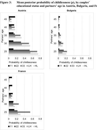
To summarise our knowledge about the influence of couples’ educational status on their reproductive behaviour, the mean posterior probability of childlessness and the expected number of children by couples’ varying educational profiles and partners’ age are presented in Figures 3‒4.6 Both measures are computed assuming that the female
and male partner are of the same age. All the remaining covariates are at their reference levels, and the number of rooms in the household is assumed to be equal to the typical value observed in a country (4 in Austria and France and 3 in Bulgaria).
The overall level of the probability of childlessness clearly differs in the countries analysed. The highest values, regardless of partners’ age, are observed in Austria and the lowest in Bulgaria (Figure 3). In all the countries considered, partners with low levels of education at age 25 have the lowest probability of being childless, equal to 0.116 in Austria, 0.138 in France, and only 0.021 in Bulgaria. This finding confirms that these couples start their reproductive careers sooner than other unions. In turn, the highest probability of childlessness among younger respondents belongs to homogamous highly educated partners in France (0.542), while in Austria and Bulgaria both homogamy in high education and hypogamy are associated with the highest risk of being childless (approximately 0.7 in Austria and 0.2 in Bulgaria). However, at the end of older couples’ reproductive careers the pattern changes significantly: Among all the selected profiles except for low-educated unions, the probability of childlessness gradually declines as the respondents get older. In Austria and Bulgaria, older partners
6 Expected number of children: the expected value of the hurdle Poisson distribution, equal to the product of
the probability of parenthood and the expected value of the Poisson part , scaled by∋1,exp(,κ)(,1 ‒
see equation (1).
who are low-educated have an even higher risk of childlessness than their younger counterparts. As a result, low-educated couples at the end of their reproductive careers have the highest probability of childlessness, while the difference between other profiles is much smaller than among younger respondents. Still, homogamy in high education and hypogamy in Austria and Bulgaria are connected to a higher probability of childlessness than hypergamous or homogamous medium-educated unions. However, in France, apart from low-educated unions, couples at older ages do not differ with respect to their risk of childlessness. This finding implies that the negative effect of homogamy in high education found for younger partners might possibly be attributed to the tempo rather than the quantum effect of fertility.
Figure 3: Mean posterior probability of childlessness (p), by couples’
educational status and partners’ age in Austria, Bulgaria, and France
Austria Bulgaria
France
Note: Probabilities reported in the graphs are computed on the basis of the model estimated in Table 3, assuming that the female and male partners are of the same age.
0 0.2 0.4 0.6 0.8
25 30 35 40 45
Probability of childlessness
P
ar
ne
rs
’
ag
e
11 22 33 LH HL
0 0.2 0.4 0.6 0.8
25 30 35 40 45
Probability of childlessness
P
ar
tn
er
s’
ag
e
11 22 33 LH HL
0 0.2 0.4 0.6 0.8
25 30 35 40 45
Probability of childlessness
P
ar
tn
er
s’
ag
e
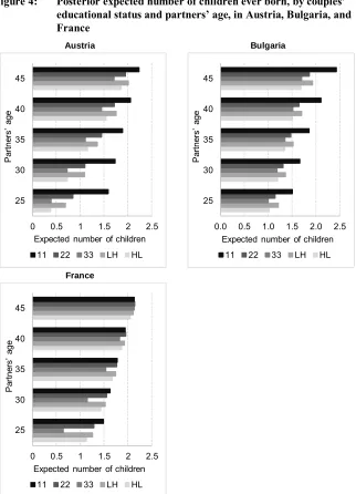
The a posteriori expected average number of children, which also takes into account the corresponding probability of childlessness, is the highest among homogamous low-educated unions, regardless of partners’ age (Figure 4). This implies that the highest fertility is, in general, observed among low-educated couples. Interestingly, the family sizes for this type of union are similar in all the countries considered, starting with a value of 1.5 children among partners aged 25 and ending with approximately 2.2 children at the age of 45. In addition, in Austria and Bulgaria the lowest fertility was found for highly educated partners, meaning that in these two countries the effect of educational level on fertility is clearly negative. In Austria, among all types of unions but the low-educated, the results obtained for the youngest couples suggest a noteworthy postponement of childbearing as compared to other countries, which very probably will also have an impact on their future completed family sizes. In Bulgaria, in turn, the negative effect of hypogamy on fertility among the oldest couples is much more evident than in other countries: Only half of hypogamous partners have two children on average at age 45, while the other half finished their reproduction after one child. This effect is similar to the effect of homogamy in high education. Moreover, as shown in Table A-4 in the Appendix, this negative effect of hypogamy is mainly attributed to couples in which the female partner is tertiary-educated and the male partner has a medium educational level. As a consequence, the effect might be assigned to the negative impact of a high female educational level. Regarding highly educated couples, the results indicate that their postponement is smallest in Bulgaria, resulting in them having one child on average at the age of 25. Finally, in France the substantial postponement of childbearing is notable among the 25-year-old highly educated partners, but since the difference between the completed fertility of the oldest respondents of all educational levels is negligible it is very likely that the highly educated will ‘catch up’ at older ages.
Figure 4: Posterior expected number of children ever born, by couples’ educational status and partners’ age, in Austria, Bulgaria, and France
Austria Bulgaria
France
Note: Expected number of children reported in the graphs are computed on the basis of the model estimated in Table 3, assuming that the female and male partner are of an equal age.
0 0.5 1 1.5 2 2.5
25 30 35 40 45
Expected number of children
P
ar
tn
er
s’
ag
e
11 22 33 LH HL
0.0 0.5 1.0 1.5 2.0 2.5
25 30 35 40 45
Expected number of children
P
ar
tn
er
s’
ag
e
11 22 33 LH HL
0 0.5 1 1.5 2 2.5
25 30 35 40 45
Expected number of children
P
ar
tn
er
s’
ag
e
Regarding control covariates, household monthly income is negatively associated with couples’ number of children in Bulgaria, while no significant impact is revealed in France. In Austria the results are mixed: On the one hand, a high household income is connected to a higher probability of being childless, but on the other hand low income is correlated with a lower number of children among parents. Hours worked per week by a woman are, in general, negatively correlated with the probability of childlessness, which means that working less is associated with higher chances of parenthood. This effect is the strongest in Austria, where not working is also connected to a higher number of children. However, the group of women who do not work (zero hours worked per week) also includes those on maternity leave, which may partially explain the association found for the “none” working-hours level. As for the ages of the woman and man, both covariates are positively correlated with fertility in all the analysed countries, meaning that the older the woman or man the lower the chance of childlessness and the higher the number of children ever born. Type of settlement, in general, does not influence fertility: The only significant effect is in Bulgaria, where living in a rural area increases the number of children. Partners who cohabit have a higher chance of childlessness and a lower number of children ever born: They clearly postpone having children or want to have fewer offspring more often. The number of rooms in the house (flat) is positively correlated with couples’ fertility. Couples where the woman is a housewife have a lower probability of childlessness in France and a higher number of children in both France and Austria. Finally, in the parenthood state, benefiting from institutional childcare is associated with having more children for Austrian and Bulgarian couples but not for French couples.
5. Robustness checks
5.1 Measures of education
This study concentrates on the effect of partners’ educational (in)equality on the number of children ever born. The way of measuring educational homogamy and heterogamy between partners is always a subject of discussion. The robustness of the results according to different measures of educational endogamy is presented below. All models are compared to Model 1, which is the basic model that includes couples’ educational status (Measure 1) and all control covariates, but no interactions (see Table A-1 in the Appendix).
main model specification. However, the influence of male and female education was examined in Model 2 and the results are given in Table A-2 in the Appendix. In general, both female and male education is negatively correlated with reproductive behaviour. However, women’s education has the stronger impact on couples’ fertility, and its negative effect is coherent with microeconomic theory and many previous findings.
Secondly, there are competing ways to measure educational endogamy. Individual levels of education are coded in the GGS dataset using the ISCED-97 classification. Seven levels, from 0 (preprimary education) to 6 (second stage of tertiary education), are distinguished. The previously considered approach (Measure 1) treats similar educational levels as equal, so, for example, a woman with a PhD and a man with a master’s degree are considered as a homogamous highly educated couple. The other, ‘precise’ approach (Measure 3) is to distinguish all possible heterogamy between partners, so that, for example, a woman with a doctoral degree and a man with a master’s degree represent a hypogamous couple. In view of this the following groups are distinguished: eduLL – both partners have homogamous levels of low education (ISCED code pairings 0‒0, 1‒1, and 2‒2); eduMM – partners with homogamous medium educational levels (pairings of 3–3 and 4–4); eduHH – partners with homogamous high education (pairings 5–5 and 6–6); eduHYPER – hypergamy, the female partner has a lower education level than the male partner (woman’s education given in ISCED number is lower than the man’s); and eduHYPO – hypogamy, the female partner has a higher education level than the male partner (woman’s ISCED number is higher than the man’s). Model 3 replaces the previously used couples’ educational status with the measure of educational constellations described above (Table A-3 in the Appendix). The results confirm that the effect of partners’ educational (in)equality is robust on different measures of educational endogamy. The only difference provided by Model 3 compared to Model 1 is the statistically significant positive influence of hypergamous unions on the number of children among parents in Bulgaria.
gap between partners reveals more detailed relationships with fertility (Table A-4 in the Appendix). The educational hypogamy type edu32 clearly restrains having a first child in all the analysed countries and limits the number of children among parents in Bulgaria. Hypergamy type edu13 increases the probability of being childless in France, while type edu12 enhances the fertility of parents in Austria.
5.2 Model comparison
Models with different measures of partners’ educational status (Models 1, 2, 3, and 4) were compared using posterior odds (PO) (see, e.g., Lancaster 2004). The posterior odds ratio of two competitive models is equal to the Bayes factor7 (BF) multiplied by
the prior odds ratio of these models. In the case of equal prior chances of the competitive models, the posterior odds ratio is reduced to the Bayes factor. Prior odds are proportional to the function of2 , where stands for the number of the model’s parameters. Thus, models with a lower number of parameters have a priori higher probability. Since Models 1, 2, and 3 have the same number of parameters ( , , equal to 33) the prior chances of each of these models are equal. Model 4 has more parameters than Model 1 ( = 41), therefore its prior chance is equal to the ratio of
2 ( )= 2 . The positive (negative) values of the logarithms of PO mean that the
posterior probability of Model 1 is10 ( ) times greater (smaller) than the probability
of the competitive model, e.g., in the case of Bulgaria, Model 1 is a posteriori
10 . ≈ 1228 times more probable than Model 3 (Table A-5 in the Appendix). Based
on the results of model comparison, we conclude that Measure 1 is, in general, similar to or better than the rest of the considered measures. The only significant improvement is achieved by Model 2 (separate partners’ educational level) in Austria, where, in light of the data, it turned out to be more probable than Model 1 (log of posterior odds of ‒ 2.125).
5.3 Control covariates
As mentioned in section 3.1, several control variables included in the model may be the consequence of realized fertility, rather than its determinants. These are: household income, female working hours, number of rooms, being a housewife, and institutional
7 According to Lancaster (2004: 98) the Bayes factor “is the ratio of the prior probabilities of the data under
help with childcare. The robustness of the results due to the inclusion or exclusion of these possibly endogenous covariates was considered. Five additional models were built for each country, each lacking one of the five covariates mentioned above. All the remaining covariates were included as in Model 1. The impact of couples’ educational status on their number of children remains coherent, regardless of the model (table with results available on request).
6. Conclusions
In this paper we focus on the impact of educational equality or inequality between partners and their joint level of educational resources on their number of children ever born. We allow other drivers of childlessness and having children by applying the hurdle zero-truncated Poisson model. Using GGS data for Austria, Bulgaria, and France, we observe couples with female partners aged 24‒45 and examine how their number of children ever born varies according to partners’ educational constellations. The three chosen countries provide different conditions for work–family life balance. Among European countries, Austria has a medium level of gender equality and low unemployment but an insufficient childcare system. When Bulgaria was a socialist state the dual-earner family model prevailed, but after the collapse of the regime female labour force participation declined. A relatively low level of gender equality and unadjusted family institutions also characterize Bulgaria. In France the level of gender equality is similar to Austria’s and the childcare system is one of the best in Europe.
positive impact of low education might be explained by enlarging families sooner than other unions do, but also, as revealed for couples with almost completed fertility, the quantum effect might be crucial.
As for educational hypogamy, the general conclusion is that it has a negative impact on couples’ reproductive behaviour, but only in Bulgaria and Austria; again, no significant effect was found in France. Partnerships in which the female is more highly educated than the male have a higher posterior probability of childlessness in both countries, and in Bulgaria a lower number of children on average. However, these effects are mainly induced by unions of highly educated women with medium-educated men, which suggests a negative impact of a high female educational level. Hypergamous couples in general do not significantly differ from their homogamous medium-educated counterparts. However, when different levels of hypergamy were considered it was found that in France, unions of low-educated women with highly educated men do postpone the first birth or, more often, stay childless, while in Austria, partnerships in which the woman is low-educated and a man has a medium educational level have a higher risk of enlarging their family after becoming parents than a medium-educated couple.
The main conclusion regarding the country-specific impact of couples’ education on their reproductive behaviour is that the association between fertility and couple’s educational status is highly sensitive to context. In Austria and Bulgaria the level of a couple’s educational resources seems to play a major role in determining its fertility behaviour, while the small variation in fertility due to couple-level education observed in France indicates that an adequate childcare system and school organisation, accompanied by a proper level of gender equality, might decrease the female opportunity cost of childbearing, help couples overcome possible obstacles, and enhance fertility at all educational profiles.
7. Acknowledgements
References
Abel, G.J., Bijak, J., Findlay, A., McCollum, D., and Wiśniowski, A. (2013). Forecasting environmental migration to the United Kingdom: An exploration using Bayesian models. Population and the Environment 35(2): 183–203.
doi:10.1007/s11111-013-0186-8.
Anderson, T. and Kohler, H.-P. (2015). Low fertility, socioeconomic development, and gender equity. Population and Development Review 41(3): 381–407.
doi:10.1111/j.1728-4457.2015.00065.x.
Anttonen, A. and Sipilä, J. (1996). European social care services: Is it possible to identify models? Journal of European Social Policy 6(2): 87–100. doi:10.1177/09 5892879600600201.
Barthold, J.A., Myrskylä, M., and Jones, O.R. (2012). Childlessness drives the sex difference in the association between income and reproductive success of modern Europeans. Evolution and Human Behavior 33(6): 628‒638.
doi:10.1016/j.evolhumbehav.2012.03.003.
Baudin, T. (2015) Religion and fertility: The French connection. Demographic Research32(13): 397‒420.doi:10.4054/DemRes.2015.32.13.
Baudin, T., de la Croix, D., and Gobbi, P. (2015). Fertility and childlessness in the United States. American Economic Review 105(6): 1852‒1882. doi:10.1257/ aer.20120926.
Baudin, T., de la Croix, D., and Gobbi, P. (2014). Development policies when accounting for the extensive margin of fertility. IRES working paper. Louvain: Université Catholique de Louvain.
Bauer, G. and Jacob, M. (2009). The influence of partners’ education on family formation. EQUALSOC Working Paper 2009/4.
Bauer, G. and Kneip, T. (2013). Fertility from a couple perspective: A test of competing decision rules on prospective behaviour. European Sociological Review 29(3): 535‒548.doi:10.1093/esr/jcr095.
Becker, G.S. (1960). An economic analysis of fertility. In:Demographic and economic change in developed countries. National Bureau of Economic Research Conference Series 11. New York: Columbia University Press: 209‒231.
Begall, K. (2013). How do educational and occupational resources relate to the timing of family formation? A couple analysis of the Netherlands. Demographic Research 29(34): 907‒936.doi:10.4054/DemRes.2013.29.34.
Begall, K. and Mills, M. (2013). The influence of educational field, occupation, and occupational sex segregation on fertility in the Netherlands. European Sociological Review 29(4): 720‒742.doi:10.1093/esr/jcs051.
Bijak, J. (2011). Forecasting international migration in Europe. A Bayesian view. Springer Series on Demographic Methods and Population Analysis, vol. 24.
doi:10.1007/978-90-481-8897-0.
Bijak, J. and Bryant, J. (2016). Bayesian demography 250 years after Bayes.Population Studies 70(1): 1‒19.doi:10.1080/00324728.2015.1122826.
Bryant, J. and Graham, P. (2013). Bayesian demographic accounts: Subnational population estimation using multiple data sources.Bayesian Analysis 8(3): 591‒ 622.doi:10.1214/13-BA820.
Brzozowska, Z. (2014). Fertility and education in Poland during state socialism.
Demographic Research 31(12): 319–336.doi:10.4054/DemRes.2014.31.12. Cameron, A.C. and Trivedi, P.K. (1998).Regression analysis of count data. New York:
Cambridge University Press.doi:10.1017/CBO9780511814365.
Cronk, L. (1991). Wealth, status, and reproductive success among the Mukogodo of Kenya. American Anthropologist 93(2): 345–360. doi:10.1525/aa.1991.93. 2.02a00040.
Doepke, M. and Kindermann, F. (2016). Bargaining over babies: Theory, evidence, and policy implications. National Bureau of Economic Research Working Paper (No. w22072).doi:10.3386/w22072.
Esping-Andersen, G. (1990).The three worlds of welfare capitalism. Cambridge: Polity Press. Esping-Andersen, G. and Billari, F.C. (2015). Re-theorizing family demographics.
Population and Development Review 41(1): 1–31. doi:10.1111/j.1728-4457. 2015.00024.x.
Fieder, M. and Huber, S. (2007). The effects of sex and childlessness on the association between status and reproductive output in modern society.Evolution and Human Behavior 28(6): 392–398.doi:10.1016/j.evolhumbehav.2007.05.004.
Demographic Research 19(7): 139–170 (Special Collection 7: Childbearing Trends and Policies in Europe).doi:10.4054/DemRes.2008.19.7.
Generations and Gender Programme (2015). Dataset. http://www.ggp-i.org/data/data-access.html.
Gerster, M., Keiding, N., Knudsen, L. B., and Strandberg-Larsen, K. (2007). Education and second birth rates in Denmark 1981‒1994. Demographic Research 17(8): 181‒210.doi:10.4054/DemRes.2007.17.8
Goldscheider, F., Bernhardt, E., and Lappegård, T. (2015). The gender revolution: A framework for understanding changing family and demographic behavior.
Population and Development Review 41(2): 207–239. doi:10.1111/j.1728-4457.2015.00045.x.
Gurven, M. and von Rueden, C. (2006). Hunting, social status and biological fitness.
Biodemography and Social Biology 53(1‒2): 81–99. doi:10.1080/19485565. 2006.9989118.
Jalovaara, M. and Miettinen, A. (2013). Does his paycheck also matter? The socioeconomic resources of co-residential partners and entry into parenthood in Finland. Demographic Research 28(31): 881–916. doi:10.4054/DemRes.2013. 28.31.
Kan, M.Y., Sullivan, O., and Gershuny, J. (2011). Gender convergence in domestic work: Discerning the effects of international and institutional barriers from large-scale data.Sociology 45(2): 234‒251.doi:10.1177/0038038510394014. Koytcheva, E. and Philipov, D. (2008). Bulgaria: Ethnic differentials in rapidly declining
fertility. Demographic Research 19(13): 361–402. doi:10.4054/DemRes. 2008.19.13.
Kravdal, Ø. and Rindfuss, R.R. (2008). Changing relationships between education and fertility: A study of women and men born 1940 to 1964.American Sociological Review73(5): 854‒873.doi:10.1177/000312240807300508.
Kreyenfeld, M. (2004). Fertility decisions in the FRG and GDR: An analysis with data from the German Fertility and Family Survey.Demographic Research SC3(11): 275–318.doi:10.4054/DemRes.2004.S3.11.
Lappegård, T. and Rønsen, M. (2005). The multifaceted impact of education on entry into motherhood. European Journal of Population 21(1): 31–49. doi:10.1007/ s10680-004-6756-9.
Lesthaeghe, R. and Permanyer, I. (2014). European sub-replacement fertility: Trapped or recovering? PSC Research Report No. 14‒822, June 2014.
Lesthaeghe, R. and van de Kaa, D. (1986). Twee Demografische Transities? In: Lesthaeghe, R. and van de Kaa, D. (eds.). Groei of Krimp? Book volume of ‘Mens en Maatschappij’. Deventer: Van Loghum-Slaterus: 9‒24.
Liefbroer, A.C. and Corijn, M. (1999). Who, what, where, and when? Specifying the impact of educational attainment and labour force participation on family formation. European Journal of Population 15(1): 45–75. doi:10.1023/A:100 6137104191.
Long, J.S. and Freese, J. (2006).Regression models for categorical dependent variables using Stata. College Station: Stata Press.
Mason, K.O. (1997). Gender and demographic change : What do we know? In: Jones, G.W., Douglas, R.M., Caldwell, J.C., and D’Souza, R.M. (eds.).The continuing demographic transition. Oxford: Oxford University Press: 158‒182.
Matysiak, A. and Vignoli, D. (2008). Fertility and women’s employment: A meta-analysis.European Journal of Population 24(4): 363‒384. doi:10.1007/s10680-007-9146-2.
McDonald, P. (2000). Gender equity, social institutions and the future of fertility.
Journal of Population Research 17(1): 1–16.doi:10.1007/BF03029445.
Neyer, G. (2003). Family policies and low fertility in Western Europe. Journal of Population and Social Security 1(Suppl.): 46‒93.
OECD (2016). OECD family database [electronic resource]. Paris: OECD, Social Policy Division, Directorate of Employment, Labour and Social Affairs. www.oecd.org/social/family/database
Oppenheimer, V.K. (1994). Women’s rising employment and the future of the family in industrial societies. Population and Development Review 20(2): 293–342.
doi:10.2307/2137521.
Osiewalska, B. (2015). Couples’ socioeconomic resources and competed fertility in Poland.Studia Demograficzne1(167): 31‒60.
Pohlmeier, W. and Ulrich, V. (1995). An econometric model of the two-part decision making process in the demand for health care. Journal of Human Resources
30(2): 339–361.doi:10.2307/146123.
Raftery, A.E., Li, N., Ševčíková, H., Gerland, P., and Heilig, G.K. (2012). Bayesian probabilistic population projections for all countries. Proceedings of the National Academy of Sciences USA 109(35): 13915–13921. doi:10.1073/pnas. 1211452109.
Schmertmann, C., Zagheni, E., Goldstein, J.R., and Myrskylä, M. (2014). Bayesian forecasting of cohort fertility. Journal of the American Statistical Association
109(506): 500–513.doi:10.1080/01621459.2014.881738.
Skirbekk, V. (2008). Fertility trends by social status. Demographic Research 18(5): 145–180.doi:10.4054/DemRes.2008.18.5.
Sobotka, T. (2015). Low fertility in Austria and the Czech Republic: Gradual policy adjustments. Vienna Institute of Demography Working Papers (No. 2/2015).
Van Bavel, J. (2012). The reversal of gender inequality in education, union formation and fertility in Europe. Vienna Yearbook of Population Research 10: 127–154.
doi:10.1553/populationyearbook2012s127.
Vignoli, D., Drefahl, S., and De Santis, G. (2012). Whose job instability affects the likelihood of becoming a parent in Italy? A tale of two partners. Demographic Research26(2): 41‒62.doi:10.4054/DemRes.2012.26.2.
Von Rueden, C., Gurven, M., and Kaplan, H. (2011). Why do men seek status? Fitness payoffs to dominance and prestige.Proceedings of the Royal Society of London B: Biological Sciences 278(1715): 2223–2232.doi:10.1098/rspb.2010.2145. Winkler-Dworak, M. and Toulemon, L. (2007). Gender differences in the transition to
adulthood in France: Is there convergence over the recent period? European Journal of Population 23(3–4): 273–314.doi:10.1007/s10680-007-9128-4. Wiśniowski, A., Smith, P.W.F., Bijak, J., Raymer, J., and Forster, J.J. (2015). Bayesian
population forecasting: extending the Lee‒Carter method. Demography 52(3): 1035‒1059.doi:10.1007/s13524-015-0389-y.
Appendix
Table A-1: The main measure of couples’ educational status – similar partners’ educational levels treated as equal (Measure 1)
Model 1
Childlessness (p) Parenthood(λ) Austria
(MS)
Bulgaria (MS)
France (MS)
Austria (MS)
Bulgaria (MS)
France (MS) Educational status of couple
edu11 ‒0.584 (0.130) ‒1.373 (0.006) 0.411 (0.116) 0.405 (0.000) 0.459 (0.00) 0.091 (0.121) edu33 0.817 (0.001) 0.550 (0.032) 0.955 (0.001) ‒0.170 (0.036) ‒0.156 (0.036) ‒0.170 (0.016) eduLH 0.074 (0.365) ‒0.387 (0.199) 0.051 (0.434) 0.052 (0.186) 0.061 (0.229) ‒0.025 (0.347) eduHL 0.960 (0.001) 0.425 (0.060) 0.388 (0.072) ‒0.006 (0.478) ‒0.177 (0.009) ‒0.061 (0.194) Household income Low ‒0.288 (0.084) ‒0.762 (0.018) 0.038 (0.424) ‒0.102 (0.045) 0.146 (0.009) 0.071 (0.103) High 0.704 (0.007) ‒0.038 (0.447) 0.401 (0.150) ‒0.054 (0.261) ‒0.037 (0.307) 0.011 (0.446)
Female working hours
None ‒2.639 (0.000) ‒1.019 (0.002) ‒0.105 (0.351) 0.181 (0.008) 0.093 (0.075) 0.024 (0.379)
20 or fewer ‒1.797
(0.000) 0.385 (0.220) ‒0.623 (0.035) 0.076 (0.125) ‒0.077 (0.299) 0.098 (0.094)
41 or more 0.747
(0.003) 0.027 (0.453) 0.267 (0.169) 0.095 (0.177) 0.007 (0.451) ‒0.049 (0.280)
Age of woman ‒0.648
(0.000) ‒0.141 (0.012) ‒0.488 (0.002) 0.083 (0.018) 0.177 (0.000) 0.072 (0.031)
Age of man ‒0.238
(0.019) ‒0.247 (0.055) ‒0.336 (0.006) 0.069 (0.017) 0.045 (0.091) 0.067 (0.019)
Rural area 0.042
(0.407) ‒0.212 (0.235) ‒0.132 (0.256) 0.030 (0.273) 0.156 (0.007) 0.028 (0.299) Cohabitation 1.796 (0.000) 2.139 (0.000) 1.317 (0.000) ‒0.417 (0.000) 0.079 (0.194) ‒0.211 (0.002)
Number of rooms ‒0.384
(0.000) ‒0.055 (0.279) ‒0.670 (0.000) 0.067 (0.000) 0.034 (0.044) 0.118 (0.000) Housewife 0.467 (0.165) ‒0.459 (0.281) ‒2.024 (0.000) 0.205 (0.006) 0.052 (0.344) 0.296 (0.001)
Institutional help with childcare 0.152
(0.004) 0.146 (0.013) ‒0.010 (0.428) Intercept 0.715 (0.010) ‒2.429 (0.000) 0.536 (0.098) ‒0.254 (0.005) ‒0.414 (0.000) ‒0.274 (0.009)
Total sample size 448 133 316 1,922 2,789 1,831
Table A-2: Alternative measure of couples’ educational status ‒ partners’ individual levels of education (Measure 2)
Model 2
Childlessness (p) Parenthood(λ) Austria
(MS)
Bulgaria (MS)
France (MS)
Austria (MS)
Bulgaria (MS)
France (MS) Female educational level
Low ‒0.600 ‒1.251 0.171 0.233 0.320 0.039
(0.032) (0.008) (0.252) (0.001) (0.000) (0.243)
High 0.906 0.463 0.607 ‒0.107 ‒0.204 ‒0.128
(0.000) (0.046) (0.009) (0.075) (0.005) (0.028) Male educational level
Low ‒0.021 ‒0.168 0.208 0.194 0.164 0.053
(0.478) (0.350) (0.183) (0.012) (0.013) (0.186)
High 0.138 0.127 0.577 ‒0.074 0.006 ‒0.076
(0.256) (0.336) (0.006) (0.121) (0.470) (0.134)
Household income
Low ‒0.217 ‒0.728 0.132 ‒0.130 0.134 0.050
(0.143) (0.014) (0.275) (0.015) (0.016) (0.184)
High 0.595 ‒0.066 0.367 ‒0.031 ‒0.019 0.029
(0.017) (0.414) (0.170) (0.361) (0.396) (0.366)
Female working hours
None ‒2.704 ‒0.966 ‒0.129 0.180 0.071 0.031
(0.000) (0.006) (0.317) (0.006) (0.130) (0.355)
20 or fewer ‒1.83 0.395 ‒0.630 0.070 ‒0.066 0.104
(0.000) (0.220) (0.036) (0.140) (0.328) (0.087)
41 or more 0.706 0.058 0.265 0.091 ‒0.014 ‒0.047
(0.006) (0.416) (0.169) (0.185) (0.412) (0.290)
Age of woman ‒0.651 ‒0.423 ‒0.486 0.085 0.180 0.065
(0.000) (0.013) (0.002) (0.016) (0.000) (0.047)
Age of man ‒0.233 ‒0.250 ‒0.321 0.065 0.038 0.070
(0.026) (0.050) (0.007) (0.022) (0.128) (0.016)
Rural area 0.055 ‒0.099 ‒0.101 0.031 0.115 0.023
(0.382) (0.375) (0.309) (0.267) (0.026) (0.329)
Cohabitation 1.777 2.193 1.318 ‒0.416 0.065 ‒0.219
(0.000) (0.000) (0.000) (0.000) (0.245) (0.002)
Number of rooms ‒0.399 ‒0.060 ‒0.685 0.069 0.032 0.120
(0.000) (0.271) (0.000) (0.000) (0.055) (0.000)
Housewife 0.661 ‒0.451 ‒1.980 0.184 0.067 0.293
(0.086) (0.285) (0.001) (0.012) (0.294) (0.002)
Institutional help with childcare 0.168 0.151 0.006
(0.003) (0.011) (0.455)
Intercept 0.825 ‒2.432 0.369 ‒0.263 ‒0.400 ‒0.278
(0.005) (0.000) (0.186) (0.003) (0.000) (0.006)
Table A-3: Alternative measure of couples’ educational status – precise educational endogamy (Measure 3)
Model 3
Childlessness (p) Parenthood(λ) Austria
(MS)
Bulgaria (MS)
France (MS)
Austria (MS)
Bulgaria (MS)
France (MS) Couples’ educational status
eduLL ‒0.498 ‒1.419 0.230 0.388 0.383 0.114
(0.177) (0.006) (0.287) (0.001) (0.000) (0.094)
eduHH 0.702 0.528 0.953 ‒0.176 ‒0.143 ‒0.151
(0.009) (0.034) (0.001) (0.046) (0.050) (0.034)
eduHYPER 0.117 ‒0.452 0.370 0.022 0.148 ‒0.031
(0.301) (0.154) (0.094) (0.347) (0.026) (0.319)
eduHYPO 0.726 0.419 0.432 0.029 ‒0.124 ‒0.086
(0.001) (0.059) (0.053) (0.337) (0.042) (0.099)
Household income
Low ‒0.249 ‒0.854 ‒0.046 ‒0.101 0.191 0.078
(0.121) (0.009) (0.405) (0.043) (0.002) (0.075)
High 0.787 ‒0.040 0.438 ‒0.063 ‒0.041 ‒0.005
(0.004) (0.445) (0.122) (0.229) (0.292) (0.479)
Female working hours
None ‒2.668 ‒1.079 ‒0.099 0.182 0.113 0.022
(0.000) (0.002) (0.349) (0.008) (0.040) (0.385)
20 or fewer ‒1.783 0.411 ‒0.592 0.075 ‒0.069 0.087
(0.000) (0.202) (0.033) (0.122) (0.321) (0.119)
41 or more 0.806 ‒0.008 0.245 0.100 0.005 ‒0.049
(0.003) (0.491) (0.196) (0.164) (0.464) (0.276)
Age of woman ‒0.625 ‒0.426 ‒0.490 0.081 0.186 0.068
(0.000) (0.012) (0.001) (0.018) (0.000) (0.039)
Age of man ‒0.241 ‒0.241 ‒0.339 0.072 0.038 0.070
(0.019) (0.063) (0.005) (0.015) (0.123) (0.014)
Rural area ‒0.021 ‒0.251 ‒0.164 0.029 0.176 0.033
(0.456) (0.200) (0.210) (0.292) (0.003) (0.258)
Cohabitation 1.806 2.104 1.315 ‒0.418 0.125 ‒0.216
(0.000) (0.000) (0.000) (0.000) (0.093) (0.002)
Number of rooms ‒0.389 ‒0.053 ‒0.677 0.066 0.029 0.118
(0.000) (0.285) (0.000) (0.000) (0.067) (0.000)
Housewife 0.463 ‒0.397 ‒2.006 0.214 0.050 0.293
(0.163) (0.324) (0.000) (0.004) (0.351) (0.001)
Institutional help with childcare 0.146 0.143 ‒0.020
(0.006) (0.017) (0.360)
Intercept 0.686 ‒2.404 0.593 ‒0.253 ‒0.415 ‒0.266
(0.018) (0.000) (0.066) (0.007) (0.000) (0.008)
Table A-4: Alternative measure of couples’ educational status – levels of educational heterogamy (Measure 4)
Model 4
Childlessness (p) Parenthood(λ) Austria
(MS)
Bulgaria (MS)
France (MS)
Austria (MS)
Bulgaria (MS)
France (MS) Couples’ educational status
edu11 ‒0.686 ‒1.439 0.375 0.415 0.476 0.105
(0.103) (0.004) (0.146) (0.000) (0.000) (0.089)
edu33 0.837 0.570 0.983 ‒0.188 ‒0.168 ‒0.176
(0.001) (0.029) (0.000) (0.027) (0.025) (0.011)
HYPER edu13 ‒0.018 ‒0.105 0.878 0.185 0.096 ‒0.042
(0.503) (0.455) (0.045) (0.116) (0.339) (0.361)
edu23 0.372 0.084 0.137 ‒0.090 ‒0.086 ‒0.139
(0.073) (0.432) (0.384) (0.108) (0.250) (0.125)
edu12 ‒0.485 ‒0.758 ‒0.359 0.174 0.128 0.018
(0.083) (0.103) (0.167) (0.014) (0.101) (0.397)
HYPO edu31 0.499 ‒0.143 0.464 ‒0.058 ‒0.102 ‒0.133
(0.289) (0.444) (0.110) (0.400) (0.332) (0.116)
edu32 1.186 0.482 0.556 ‒0.078 ‒0.236 ‒0.124
(0.000) (0.049) (0.042) (0.223) (0.005) (0.095)
edu21 0.136 0.197 ‒0.043 0.115 ‒0.029 0.056
(0.380) (0.331) (0.462) (0.170) (0.393) (0.266)
Household income
Low ‒0.218 ‒0.745 0.113 ‒0.124 0.135 0.050
(0.153) (0.019) (0.293) (0.022) (0.015) (0.185)
High 0.638 ‒0.075 0.384 ‒0.036 ‒0.024 0.023
(0.011) (0.398) (0.158) (0.338) (0.369) (0.396)
Female working hours
None ‒2.707 ‒1.006 ‒0.119 0.182 0.083 0.028
(0.000) (0.004) (0.333) (0.007) (0.092) (0.362)
20 or fewer ‒1.823 0.405 ‒0.625 0.072 ‒0.074 0.101
(0.000) (0.221) (0.041) (0.126) (0.301) (0.086)
41 or more 0.713 0.035 0.260 0.091 ‒0.002 ‒0.049
(0.007) (0.450) (0.185) (0.196) (0.483) (0.282)
Age of woman ‒0.653 ‒0.415 ‒0.491 0.084 0.176 0.067
(0.000) (0.012) (0.001) (0.018) (0.000) (0.044)
Age of man ‒0.232 ‒0.253 ‒0.318 0.067 0.045 0.069
(0.021) (0.051) (0.006) (0.023) (0.092) (0.016)
Rural area 0.054 ‒0.173 ‒0.125 0.026 0.138 0.025
(0.381) (0.284) (0.277) (0.312) (0.010) (0.312)
Cohabitation 1.788 2.184 1.342 ‒0.417 0.072 ‒0.217
(0.000) (0.000) (0.000) (0.000) (0.219) (0.003)
Number of rooms ‒0.398 ‒0.056 ‒0.682 0.069 0.034 0.118
(0.000) (0.287) (0.000) (0.000) (0.040) (0.000)
Housewife 0.641 ‒0.389 ‒1.994 0.187 0.053 0.294
(0.088) (0.299) (0.001) (0.010) (0.340) (0.001)
Institutional help with childcare 0.166 0.152 0.001
(0.002) (0.012) (0.496)
Intercept 0.766 ‒2.449 0.521 ‒0.254 ‒0.405 ‒0.272
(0.009) (0.000) (0.087) (0.005) (0.000) (0.007)
Table A-5: Logarithms of posterior odds ratios of Model 1 versus other competitive models
Log10(PO)
Austria Bulgaria France
Model 1 vs Model 2 ‒2.125 0.132 ‒0.463
Model 1 vs Model 3 1.031 3.089 1.379