DEMOGRAPHIC RESEARCH
A peer-reviewed, open-access journal of population sciences
DEMOGRAPHIC RESEARCH
VOLUME 33, ARTICLE 28, PAGES 801–840
PUBLISHED 21 OCTOBER 2015
http://www.demographic-research.org/Volumes/Vol33/28/ DOI: 10.4054/DemRes.2015.33.28
Research Article
The sensitivity analysis of population
projections
Hal Caswell
Nora S´anchez Gassen
c
2015 Hal Caswell & Nora S´anchez Gassen.
1 Introduction 802
1.1 Sensitivity and elasticity 803
2 Projection as a matrix operation 804
2.1 Dynamics 804
2.2 Scenarios and parameters 806
3 Perturbation analysis of projections 807
3.1 Matrix calculus notation 807
3.2 One-sex projections 808
3.3 Two-sex projections 809
3.4 Parameters and the derivatives of matrices 810
3.5 Choosing a dependent variable 812
3.6 Aggregating perturbations over age and time 815 4 A projection of the population of Spain 817 5 Sensitivity and elasticity of the population projection of Spain 818 5.1 Sensitivity of the total population size 819 5.2 Elasticity of male and female population sizes 820 5.3 Elasticity of the school-age population (6 to 16 years) 821 5.4 Elasticity of population with dementia 823 5.5 Elasticity of dependency and support ratios 824
6 Discussion 826
6.1 Sensitivity analysis and scenarios 826
6.2 Sensitivity and uncertainty 827
6.3 Immigration and emigration 828
6.4 Data requirements and applications 829
7 Acknowledgements 830
References 831
Appendices 835
Appendix A Derivations 835
A.1 Derivatives ofn(t) 835
A.2 Derivatives of projection matrices 837
A.3 Derivatives of dependent variables 838
The sensitivity analysis of population projections
Hal Caswell1
Nora S´anchez Gassen2
Abstract
BACKGROUND
Population projections using the cohort component method can be written as time-varying matrix population models. The matrices are parameterized by schedules of mortality, fer-tility, immigration, and emigration over the duration of the projection. A variety of de-pendent variables are routinely calculated (the population vector, various weighted popu-lation sizes, dependency ratios, etc.) from such projections.
OBJECTIVE
Our goal is to derive and apply theory to compute the sensitivity and the elasticity (propor-tional sensitivity) of any projection outcome to changes in any of the parameters, where those changes are applied at any time during the projection interval.
METHODS
We use matrix calculus to derive a set of equations for the sensitivity and elasticity of any vector valued outcomeξ(t)at timetto any perturbation of a parameter vectorθ(s)at any times.
RESULTS
The results appear in the form of a set of dynamic equations for the derivatives that are integrated in parallel with the dynamic equations for the projection itself. We show re-sults for single-sex projections and for the more detailed case of projections including age distributions for both sexes. We apply the results to a projection of the population of Spain, from 2012 to 2052, prepared by the Instituto Nacional de Estad´ıstica, and deter-mine the sensitivity and elasticity of (1) total population, (2) the school-age population, (3) the population subject to dementia, (4) the total dependency ratio, and (5) the eco-nomic support ratio.
1Institute for Biodiversity and Ecosystem Dynamics (IBED), University of Amsterdam, The Netherlands.
E-Mail: [email protected].
2Institute for Biodiversity and Ecosystem Dynamics (IBED), University of Amsterdam, The Netherlands.
CONCLUSIONS
Writing population projections in matrix form makes sensitivity analysis possible. Such analyses are a powerful tool for the exploration of how detailed aspects of the projection output are determined by the mortality, fertility, and migration schedules that underlie the projection.
1. Introduction
Fifty years ago, in the first issue of the first volume of the then-new journal Demogra-phy, Nathan Keyfitz described the “population projection as a matrix operator” (Keyfitz 1964). He showed that population projections using the cohort component method could be written as matrix population models, and emphasized the value in doing so to focus attention on the mathematical structure of the projection, inviting deeper analyses of its properties with more powerful mathematical tools. Today, official projections are often implemented as computer algorithms, the details of which are obscure, but which permit almost endless fine-tuning of relationships. But the advantages of considering projections as matrix operators are no less real. In this paper, we carry on in this spirit, using matrix calculus methods to develop a thorough perturbation analysis of population projections.
As is customary in demography, we use the termprojectionto describe a conditional prediction of population size and structure, over a specified time horizon, such as are regularly developed by national governments, international consortia (e.g., Eurostat), and non-governmental organizations (U.N.). All projections are conditional in the sense that they are based on one or more hypothetical scenarios defining future rates of mortality, fertility, and migration (collectively, the “vital rates”), and also conditional on an initial population.
The vital rate scenarios are defined in terms of a set of parameters; the nature of those parameters will depend on the details of the scenarios. Sensitivity analysis (also called perturbation analysis) asks how the results of the projection would change in re-sponse to changes in the parameters. Sensitivity analysis is useful because:
1. It can project the consequences of changes in the vital rates. Such changes could result from human actions, either intentional (e.g., policies to encourage reproduc-tion, public health interventions, or conservation strategies applied to endangered species) or unintentional (e.g., consequences of pollution or environmental degra-dation), or natural changes.
3. It can be used retrospectively to decompose observed changes in an outcome into contributions from changes in each of the parameters (Caswell 2000, 2001). 4. It can be used to identify parameters the estimation of which deserves extra
atten-tion, because they have large effects on the results.
5. It can quantify uncertainty of projection results: given the uncertainty in some pa-rameterθ, and the sensitivity of an outcome of interest to changes inθ, it is possible to approximate the resulting uncertainty in the outcome. Demographers have be-come increasingly concerned with estimating the uncertainty of projection results (Booth 2006; Ahlburg and Lutz 1998).
In this paper, we focus on projections of populations classified by age and sex. Some projections are multistate models (e.g., projections of Belgium classify individuals by age, sex, nationality, and position in the household3; projections of Sweden classify
in-dividuals by age, sex, and country of birth4). We will present the sensitivity analysis of
multistate projections in a subsequent paper.
1.1 Sensitivity and elasticity
Our approach is to calculate the derivatives of the projection results to the parameters and initial conditions. This gives the effects of small changes, gives approximate results for quite large changes, and identifies parameters with particularly large or small impacts on the results. As we will show, the parameters may include aspects of mortality, fertility, or immigration. The projection results may include a variety of different functions of the population, including measures of size, structure, and growth.
We will present results for both sensitivity and elasticity. Ifyis a function ofx, we define the sensitivity ofyto changes inxas
sensitivity= dy
dx. (1)
The elasticity ofyis the proportional sensitivity, which is
elasticity = x y
dy
dx (2)
= y
x. (3)
This gives the proportional change inyresulting from a proportional change inx. There is no standard notation for elasticities, despite their widespread use in economics and popu-lation biology. The notation used here,y/x, which parallels the notation for derivatives,
3http://statbel.fgov.be/fr/binaries/FORPOP1360 10697 F tcm326-244744.pdf
is adapted from a notation used by Samuelson (1947). Elasticities are defined only when y >0andx≥0.
In Section 2 we will write both one-sex and two-sex projections as matrix operators, and discuss the scenarios that might be involved in such projections and the parameters that might determine those scenarios. In Section 3 we will give the expressions for the sensitivities and elasticities of the population vector (abundance by age class of males, or females, or both combined) to changes in mortality, fertility, and immigration. A particularly important part of our results, in Section 3.5, is to show how the sensitivity results for the population vector can be translated directly into other dependent variables, such as weighted population size, ratios, and growth rates. The derivations of results are given in detail in Appendix A.
Our approach is to write the projection as a matrix operator, and then to use ma-trix calculus (e.g., Caswell 2007, 2008, 2009; Caswell and Shyu 2012) to derive the needed derivatives of the results to underlying parameters. These methods are easily implemented in any matrix-oriented computer language, especially MATLAB, but also R. In Section 4 we will apply the calculations to a projection of the population of Spain, using information from the Instituto Nacional de Estad´ıstica (INE). We conclude with a discussion of how these results apply to evaluating the uncertainty of projections and future developments.
Notation. Matrices are denoted by upper case bold symbols (e.g., A) and vectors by lower case bold symbols (e.g.,n). All vectors are column vectors by default. The vector xTis the transpose of the vectorx. The Hadamard, or element-by-element, product ofA andBisA◦B. The Kronecker product isA⊗B. The diagonalization operator diag(x)
creates a matrix with xon the diagonal and zeros elsewhere. The vec operator, when applied to am×nmatrixXcreates amn×1vector vecXby stacking each column of Xon top of the next. The vector1is a vector of ones, and the vectorei is theith unit vector, with a 1 in theith location and zeros elsewhere. When necessary, subscripts are attached to indicate the size of matrices or vectors; e.g.,Iωis theω×ωidentity matrix.
2. Projection as a matrix operation
2.1 Dynamics
To present the basics of projection sensitivity analysis, we begin with a simple one-sex model, but we focus most of our attention on a two-sex model that includes separate rates for males and females.
The single-sex projection can be written as
wheren(t)is a vector whose entries are the numbers of individuals in each age class or stage at timet,A(t)is a projection matrix incorporating the vital rates at timet, andb(t)
is a vector giving the number of immigrants in each age class or stage at timet. The projection begins with a specified initial condition, denotedn0, and is carried out until
some target timeT.
Two-sex projections are generalizations of (4). We define population vectors nf andnm, and projection matricesAf andAm, for females and males, respectively. We assume that reproduction is female dominant5, so all fertility is attributed to females. We
decompose the projection matrices for females and males into
Af(t) = Uf(t) +φF(t) (5)
Am(t) = Um(t) (6)
whereUdescribes transitions and survival of extant individuals andFdescribes the pro-duction of new individuals by repropro-duction.
In an age-classified model, F will have effective fertilities (including infant and maternal survival as appropriate) on the first row and zeros elsewhere. A proportionφof the offspring arefemale. This model attributes reproduction to females; hence there is no need to create separate fertility matrices for reproduction by males and females.
The male component of the population is projected by the survival matrixUm; the input of new individuals comes from the female population. The projection model be-comes
nf(t+ 1) = h
Uf(t) +φF(t) i
nf(t) +bf(t) (7)
nm(t+ 1) = Um(t)nm(t) + (1−φ)F(t)nf(t) +bm(t). (8) The formulations in equations (4), (7), and (8) are general enough to encompass all the projections typically used. The vectorncan incorporate any type of population structure considered relevant. If individuals are grouped into age classes, thenAis the familiar Leslie matrix, with survival probabilities on the subdiagonal, fertilities in the first row, and zeros elsewhere. If individuals are classified by other criteria (“stages” in common usage),Awill have the structure needed to capture transitions among stages based on physiological condition, developmental stage, socio-economic grouping, marital status, parity status, etc.
Immigration, denoted here byb(t), is a particularly challenging part of population projection. We explore the reasons for this, and some of the ways in which migration is handled, in Section 6.3. Some implementations of migration require minor modifications
5Two-sex models that do not assume dominance by one sex have been used to project animal populations (e.g.,
of equations (4)–(8), but the sensitivities are derived in the same way as what we are about to show.
2.2 Scenarios and parameters
A projection is based on a scenario of how the future might unfold. The matricesU(t)
andF(t), and the vectorb(t), describe the future dynamics of mortality, fertility, and immigration. The future being unknown, considerable ingenuity is required to construct these functions. Three major approaches seem to be used, singly or in combination.
1. Extrapolation of trends. This approach starts from the observation that some vital rates (particularly mortality and fertility rates) develop gradually over time, and extrapolates those patterns into the future. The best-known of these is perhaps the Lee-Carter model for mortality, which projects mortality with a time-series model applied to a singular value decomposition of a past record of age- and time-specific mortality rates. Recent developments include sophisticated Bayesian methods that also produce statistically rigorous uncertainty bounds (e.g., Gerland et al. 2014).
2. Assumptions and expert opinion. Future trends in vital rates are sometimes simply assumed, based on unspecified conceptual models. The projections of Eurozone countries by Eurostat, for example, are based on the assumption that the mortality and fertility of all European countries will converge to a common value by the year 2150 (Lanzieri 2009). The rates for a given country in each year are determined by interpolating between the rates at the start of the projection and the final target rates. Other studies have been based on the opinion of experts who are not directly involved in the projection process. Lutz and colleagues, for instance, have used a Delphi-method based approach to collect and aggregate external expert opinions on demographic trends in a systematic manner (Ahlburg and Lutz 1998). Expecta-tions of population members about their own lives (e.g. survey data on the expected number of children or expected remaining life expectancy) have also been used to define scenarios.
Jenouvrier et al. 2009, 2012, 2014). Similarly, projections of human populations have been based on expectations about future economic, social or environmental developments (Booth 2006).
Regardless of how the scenario of future conditions is obtained, the resulting projection depends on a set ofparameterswhich jointly determine the projection matrices and the immigration vectors. We will write this set of parameters as a vectorθ, of dimensionp. In this paper, we focus on the commonly encountered case in which the parameters are the age- and time-specific rates of mortality, fertility, and immigration:
θ(t) =
µ(t) vector of mortality rates f(t) vector of age-specific fertility b(t) immigration vector
(9)
These vectors might, in turn, be expressed as functions of a scalar quantity such as life expectancy, or a parametric model such as the Gompertz, gamma-Gompertz, or Siler models for mortality, or the Coale-Trussell function for fertility. In that case, the vectorθ would include the parameters that define those functions.
3. Perturbation analysis of projections
Our goal is to quantify the sensitivity and elasticity of projection results to the parameters inθ. To do that, we need to introduce the matrix calculus framework for derivatives of vectors (the projection output) with respect to other vectors (the parameter vector). The derivations of our results are given in detail in Appendix A.
3.1 Matrix calculus notation
Matrix calculus permits the differentiation of scalar-, vector-, or matrix-valued functions of scalar-, vector-, or matrix-valued arguments. The underlying theory is presented in detail by Magnus and Neudecker (1985); for an introductory account see Abadir and Magnus (2005). The methods have been applied to demography in a series of papers (Caswell 2006, 2007, 2008, 2010, 2012; Caswell and Shyu 2012; van Raalte and Caswell 2013; Engelman, Caswell, and Agree 2014).
Ifyis an×1vector function of them×1vectorx, then the sensitivity ofytoxis then×mJacobian matrix written as
dy
dxT =
∂y
i ∂xj
We will use the fact that this calculus satisfies the chain rule, so that ifzis a function of y, then
dz
dxT = dz
dyT dy
dxT. (11)
The elasticity, or proportional sensitivity, ofywith respect toxis then×mmatrix given by
y
xT =diag(y)
−1
dy
dxT
diag(x). (12)
We will present a series of sensitivity and elasticity relationships of the form
dξ
dθT and ξ
θT
whereξis a projection output andθ is a vector of parameters. The outputξmight be the population vectorn(t), or it might be some function ofn(e.g., a dependency ratio). The sensitivity ofξis obtained from a system of equations giving a dynamic model (i.e. a model specifying changes through time) for the derivatives of the population vector at timetto a parameter change at times
dn(t) dθT(s)
wheresis the time at which the parameter vectorθis perturbed. If there areωage classes andpparameters, then this derivative is aω×pmatrix whose(i,j)entry is the derivative ofni(t)with respect to the parameterθjat times.
3.2 One-sex projections
For simplicity, we begin with the one-sex projection (4). We consider the effects of changes in the parameters at timeson the projected population at timet, fors= 0,. . .,T andt = s,. . .,T. Changes inθ(s)obviously have no effect onn(t)at an earlier time t < s(we ignore the complications of time travel). However, a perturbation at timeswill ripple throughn(t)for all later timest > s, and our goal is to find out how.
The dynamics of the population vectorn(t)are obtained by iterating equation (4). The sensitivity ofn(t)to a change inθ(s)is obtained by iterating the dynamic equation
dn(t+ 1)
dθT(s) =A(t) dn(t) dθT(s)+ (n
T(t)⊗I
ω)
dvecA(t) dθT(s) +
db(t)
dθT(s) (13)
starting from the initial condition
dn(0)
The elasticity ofn(t)toθ(s)is, from (12), n(t)
θT(s) =diag h
n(t)i
−1 dn(t)
dθT(s) diag h
θ(s)i. (15)
The structure of (13) is common to all the sensitivity results; it contains terms involving the sensitivity at timetand terms that update that sensitivity with effects onA(t)and b(t), giving the sensitivity att+ 1:
dn(t+ 1) dθT(s)
| {z }
sensitivity att+ 1
= A(t)dn(t) dθT(s)
| {z }
sensitivity att
+ (nT(t)⊗I ω)
dvecA(t) dθT(s)
| {z }
effects viaA
+ db(t)
dθT(s).
| {z }
effects viab (16)
3.3 Two-sex projections
The sensitivity of the two-sex projection is given by the two derivatives,
dnf(t) dθT(s) and
dnm(t) dθT(s).
These derivatives are obtained from dynamic expressions, for the female population
dnf(t+ 1) dθT(s) =
Uf(t) +φF(t)
dn
f(t) dθT(s)
+ nTf(t)⊗Iω
dvecUf(t) dθT(s) +φ
dvecF(t)
dθT(s)
+dbf(t)
dθT(s) (17) and the male population
dnm(t+ 1) dθT(s)
| {z }
sensitivity att+ 1
= Um(t) dnm(t)
dθT(s) + (1−φ)F(t) dnf(t) dθT(s)
| {z }
sensitivities att
+ nTm(t)⊗Iω
dvecUm(t) dθT(s)
| {z }
effects via male transitions
+ (1−φ) nTf(t)⊗Iω
dvecF(t)
dθT(s)
| {z }
effects via female fertility
+ dbm(t)
dθT(s).
| {z }
effects via immigration
Equations (17) and (18) are iterated from initial conditions
dnf(0) dθT(s) =
dnm(0)
dθT(s) =0ω×p (19)
along with the iteration of equations (7) and (8) for the population vectorsnf(t)and
nm(t).
We have labelled the terms in (18) to show the parallels with the simpler one-sex model (16). Again, the sensitivity att+ 1 depends on the sensitivity at timetand on the effects of the parameter vector on the transition and fertility matrices and on the immigration vector. In the next section we turn to the calculation of these derivatives.
The elasticities ofnf(t)andnm(t)are given by applying (15) to the corresponding derivatives for female and male population:
nf(t) θT(s) =diag
h
nf(t)
i−1dnf(t) dθT(s) diag
h
θ(s)i (20)
and similarly fornm.
The combined population of both males and females isnc =nf+nm. The sensi-tivity and elasticity ofncare
dnc(t) dθT(s) =
dnf(t) dθT(s)+
dnm(t)
dθT(s) (21)
nc(t)
θT(s) = diag h
nc(t)
i−1dnf(t) dθT(s)+
dnm(t) dθT(s)
diaghθ(s)i. (22)
The entire system of sensitivity and elasticity relationships is obtained by simultane-ously iterating equations (7) and (8) to project the populations of females and males, and the equations (17) and (18) to project the sensitivity of the female and male populations.
3.4 Parameters and the derivatives of matrices
So far we have left the parameter vectorθ undefined, because the results apply to any choice of parameter. Now we become more specific by focusing on the cases whereθis a vector of mortality rates, or of fertilities, or of immigration numbers. We consider each of these cases and present the derivatives of the matricesUandF, and the vectorb, to those parameters. These derivatives appear in the expressions (17), (18), and (21) and the corresponding elasticity equations.
A change in the parameter vectorθat timescan affect the projection matrices only whent=s; to indicate this, we will use the Kronecker delta function
δ(s,t) =
1 ifs=t
Because sex-specific mortality affects the matrices for only that sex, the following results apply to either male or female rates, so we do not include the subscript that defines the sex of the subpopulation.
• Mortality:θ=µ. Mortality rates affect the transition matrixU(or the projection matrixA, if transitions and fertility are not separated). Define the survival vector
p= exp(−µ), which appears on the subdiagonal ofU, and an indicator matrixZ
with ones on the subdiagonal and zeros elsewhere. Then
dvecA(t) dµT(s) =
dvecU(t)
dµT(s) =−δ(s,t)diag(vecZ) (Iω⊗1ω)diag p(t)
(24)
where1is a vector of ones. The derivatives ofFandbwith respect toµare zero.
• Fertility:θ =f. The fertility vector appears on the first row of the matrixF. The derivative ofFis
dvecF(t)
dfT(s) =δ(s,t) (Iω⊗e1) (25) wheree1is the first unit vector, of lengthω. The derivatives ofUandbwith
re-spect tof are zero.
• Immigration:θ=b. When the parameter vector is the immigration vector, then db(t)
dbT(s) =δ(s,t)Iω (26) and the derivatives ofU,F, andAwith respect tobare all zero.
• Initial population:θ=n0. It is also possible to calculate the sensitivity ofn(t)to
the initial population vector. The derivatives ofU,F,A, andbwith respect to the initial population are all zero, and the derivatives of the population vector reduce to an especially simple form.
Letn0,f andn0,mbe the initial male and female population vectors. The female population is independent of the initial male population, but the male population will depend on both the male and female initial populations. From equations (17) and (18) we have for the female population:
dnf(t+ 1) dnT
0,f
= (Uf(t) +φF(t))
dnf(t+ 1) dnT
0,f
(27)
with initial condition
dnf(0) dnT
0,f
For the male population, we have dependence on the initial male population
dnm(t+ 1) dnT
0,m
=Um(t) dnm(t)
dnT
0,m
(29)
with initial condition
dnm(0) dnT
0,m
=Iω. (30)
The dependence on the initial female population we have
dnm(t+ 1) dnT
0,f
=Um(t) dnm(t)
dnT
0,f
+ (1−φ)F(t)dnf(t) dnT
0,f
(31)
with initial condition
dnm(0) dnT
0,f
=0ω×ω. (32)
The behavior of these sensitivities depends on the behavior of the population and the cohorts that comprise it. From (27), it is apparent that the sensitivity of the female population to the initial female population grows or shrinks depending on whether the sequence of projection matrices, (Uf(t) +rF(t)), tends to expand or contract the population. The sensitivity of the male population to the initial male population decays according to the sequence of survival matricesU(t). Thus, in general, the sensitivity to initial population will play a greater role in rapidly expanding populations (a fact easily predictable from general principles of linear system theory). In populations that grow only slightly, or decline, over the time span of the projection, these sensitivities will be less important.
3.5 Choosing a dependent variable
These results in equations (16), (17), and (18) provide the sensitivity ofeveryage class, ateverytime from 0 toT, with respect to changes in mortality, fertility, and immigration of everyage class, ateverytime from 0 to T. This high-dimensional data structure is more information than anyone wants. It must be condensed to provide the sensitivity of specific projection outcomes of interest. An informal survey of Statistical Offices6finds
that they typically present projections of (1) the total population size, (2) the proportional representation of specific age groups (e.g., working-age adults, school-age children), (3) ratios such as the old-age, young-age, and total dependency ratios, (4) and descriptors of
6European Union, Germany, France, Belgium, Ireland, Estonia, Spain, Austria, Sweden, United Kingdom,
the age distribution such as the mean age in the population. Sometimes projections also include results on the population subject to particular diseases or handicaps.
In this section, we show how to calculate the sensitivity and elasticity of such depen-dent variables from the derivatives ofn(t)given in (17), (18), and (21). In the following, sensitivities can be applied to the female population, the male population, or the com-bined population. Derivations are given in Appendix A.3.
1. Total population sizeN(t). The total population size isN(t) =1T
ωn(t); its sensi-tivity to parameter changes at timesis
dN(t) dθT(s) =1
T ω
dn(t)
dθT(s). (33)
The elasticity ofN(t)is
N(t) θT(s)=
1 N(t)
dN(t)
dθT(s) diag(θ). (34)
2. Weighted total population size. DefineN(t) = cTn(t), wherecis a vector that applies different weights to each age class. For example,cmight contain the labor income of each age class, or the prevalence in each age class of some health con-dition.N(t)is now a weighted population size; the sensitivity ofN(t)to a change in parameters at timesis
dN(t) dθT(s) =c
Tdn(t)
dθT(s). (35)
The elasticity is again given by (34). If the weight vectorcis subject to perturba-tions (e.g., if the prevalence of a health condition were to change due to screening or treatment), the sensitivity ofN(t)to changes incis
dN(t) dcT =n
T(t). (36)
The corresponding elasticities ofN(t)tocare N(t)
cT = 1 N(t)n
T(t)diag(c). (37)
3. Ratios of weighted population sizes. Let
R(t) = a
Tn(t)
cTn(t), (38)
whereaandcare vectors of weights. The sensitivity of such a ratio (Caswell 2007) is
dR(t) dθT(s) =
cTn(t)aT−aTn(t)cT [cTn(t)]2
! dn(t)
dθT(s). (39)
The elasticity ofR(t)is
R(t) θT(s) =
1 R(t)
dR(t)
dθT(s)diag[θ(s)] . (40)
Such ratios appear frequently as dependent variables in population projections. Ex-amples include:
(a) The proportional representation of an age group (e.g., the proportion over 65 years of age). In this case,ais an indicator vector, containing ones corre-sponding to the ages in the age group, and zeros elsewhere. The vectorc=1, so thatcTNis the total population size.
(b) Dependency ratios. In this case, aandcare both indicator vectors for the relevant age groups. The old-age dependency ratio, for example, is obtained by lettingaindicate ages beyond retirement age andcindicate working ages. (c) Weighted dependency ratios. Instead of considering all individuals of retire-ment age, or working age, to be equal,aandccan be vectors of weights. For example, the economic support ratio (Prskawetz and Sambt 2014) is com-puted by lettingabe a vector giving age-specific labor income, andca vector giving age-specific consumption.
(d) Moments of the age distribution. The mean of the age distribution is obtained by setting the vectorato the midpoints of the age intervals; e.g., for one year age classes,
a= 0.5 1.5 2.5 · · · T
(41)
and settingc=1. The second moment of the age distribution is obtained by setting
a= 0.52 1.52 2.52 · · · T
(42)
(e) Moments of age-specific properties. Suppose thatB(s)is some measurement on age classx(e.g., the mean body mass index (BMI) of age classx). Then the mean BMI in the population would be obtained by settingc=1and
a= B(1) B(2) B(3) · · · T
. (43)
4. Short-term growth rates. Define thek-step growth rate of the weighted population sizecTn, at timetas
λ(t) =c
Tn(t+k)
cTn(t) . (44)
This gives the average discrete-time growth rate of the population over the nextk years, starting from yeart. The sensitivity ofλ(t)is
dλ(t) dθT(s)=
cT
cTn(t)
dn(t+k) dθT(s) −
λ(t)cT
cTn(t) dn(t)
dθT(s). (45)
The quantityλis a discrete time growth rate; the sensitivity of the corresponding continuous time, annual growth rater(t) = logλ(t)/kis
dr(t) dθT(s) =
1 kλ(t)
dλ(t)
dθT(s). (46)
3.6 Aggregating perturbations over age and time
The expressions presented so far give the response of the dependent variable at any time t, to a perturbation of any of the parameters inθ, at any other times. It is often useful to aggregate sensitivity over age, or over time, or over parameters, or all of these. Some examples are:
1. The sensitivity ofnat timetto a perturbation, at times, that affects the mortality, fertility, or immigration of all age classes by the same amount. The sensitivity of n(t)to an additive perturbation at every age is the sum of the sensitivities to the age-specific rates. The elasticity ofn(t)to a proportional perturbation at every age is the sum of the elasticities to the age-specific rates. Thus, whatever ratesθ(s)
may refer to, the sensitivity and elasticity are given by
sensitivity: dn(t)
dθT(s)1p (47)
elasticity: n(t)
2. The sensitivity of the population vector at timetto a change inθ(s)that is applied equally at every time froms = 0tos=T. A possible example of interest might be the sensitivity of the population vector in the final projection year,n(T), to a change in fertility at every age or at a specific age group over the entire projection period. In a slight abuse of notation, let us denote the sensitivity ofn(T)to this type of perturbation as
dn(T) dθT(0,T) =
T X
s=0
dn(t)
dθT(s). (49)
The corresponding elasticity is
n(t)
θT(0,T) = diag[n(t)]
−1
T X
s=0
dn(t)
dθT(s)diag[θ(s)] (50) = T X s=0
n(t)
θT(s). (51)
3. The response of a dependent variable integrated over time. For example, consider the population vector summed from time t = 0 tot = T. The sensitivity and elasticity of this sum are
d dθT(s)
T X
t=0
n(t) = T X
t=0
dn(t)
dθT(s) (52)
θT(s)
T X
t=0
n(t) = diag "
X
t
n(t) #−1 T
X
t=0
dn(t)
dθT(s)diag[θ(s)] . (53)
For example, Fox et al. (2001) projected the annual costs of care for Alzheimer’s patients in California from 2000 to 2040. They combined projections of the popu-lation over age 65 with estimates of the prevalence of various types of Alzheimer’s care and the per capita costs of such care, and transformed the annual cost figures to 1998 dollars. Although they examined the annual costs in selected years, we imagine that someone might also be interested in the accumulated expenditures, integrated over some period into the future. Denote the integrated cost fromt= 0
tot=T as
C(T) = T X
t=0
cT(t)n(t) (54)
is obtained by differentiating (54):
dC(T) dθT(s) =
T X
t=0 nT
(t) dc(t) dθT(s)+
T X
t=0 cT
(t)dn(t)
dθT(s); (55)
it includes the possible effects of the parameters on both the cost vector and the population vector. If the weighting vectorc(t)is fixed, the first term in (55) disap-pears.
4. A projection of the population of Spain
As an example, we apply the sensitivity and elasticity calculations to a projection of the population of Spain published by the Spanish Instituto Nacional de Estad´ıstica (INE). This projection is typical of cohort component projections, and Spain is an interesting case because of its recent demographic history. It has experienced rapid changes in fer-tility, mortality and migration during the past decades and today has one of the highest life expectancies and one of the lowest fertility levels within the European Union. During most of the 20th century, it was a country of emigration, but received large numbers of immigrants since the mid-1990s before recently again losing large population numbers to outmigration. Similar sudden changes in the vital rates may occur in the future and are difficult, perhaps impossible, to predict today. The sensitivity analyses can quantify the effects of changes in the vital rates that are not expected by INE today, but which would influence the projection results. Also, in contrast to many other statistical offices, INE has made the input data for their population projection freely available online. This allowed us to calculate the sensitivity analyses, and will also allow interested readers to replicate them.
The projection published by INE uses the cohort component method and distin-guishes single-year age groups (ages 0 to 100+ years) and sex of population members. It covers a 40-year period from 2012 to 2052, with a projection interval of one year (Insti-tuto Nacional de Estad´ıstica 2012a), based on the following assumptions:
• The fertility scenario is presented in the form of age-specific fertility rates. INE assumes that the total fertility rate will increase from 1.36 children per woman in 2011 to 1.56 in 2051, and that the mean age at childbearing will rise from 31 to 32 years within the same period. On their website, INE has published fertility vectors for f(t)fort = 1,. . ., 40which reflect these assumptions (Instituto Nacional de Estad´ıstica 2012b,c).
2011 to 87 years in 2051 for men, and from 83 years to 91 years for women over the same time period. Corresponding to these assumptions, INE presents a series of age- and sex-specific probabilities of death, q(t)for t = 1,. . ., 40(Instituto Nacional de Estad´ıstica 2012b,c).
• Migration assumptions are expressed in terms of age- and sex-specific immigration numbers and emigration rates. INE assumes that the migratory balance of Spain, which was negative by 50,000 persons in 2011, will recover during the projection period. In the last ten projection years, the number of persons who move to Spain is assumed to exceed emigration numbers by around 438,000 persons. Emigra-tion rates are held constant over the entire projecEmigra-tion interval (Instituto Nacional de Estad´ıstica 2012b,c).7 Because of the assumptions of INE, we incorporated
emi-gration into the matrixU, treating emigration and mortality as two competing risks for leaving the population. See Section 6.3 for further discussion of ways to treat migration.
In a press note on the population projections of 2012, INE emphasized two key findings. First, the population of Spain is expected to decline from 46.2 million persons in 2012 to 41.5 million by 2052. Second, the population is expected to age. INE estimates that 37 percent of the population will be aged 64 or older in 2052, raising the overall dependency ratio, defined as the quotient between the population under 16 and over 64 years of age and the population aged 16 to 64, from 0.504 (in 2012) to 0.995 (in 2052). These projection results form the basis of governmental planning (Instituto Nacional de Estad´ıstica 2012a). Analysing their sensitivity and elasticity to changes in the underlying assumptions is therefore not only relevant for the demographic research community, but also for policy makers in Spain.
5. Sensitivity and elasticity of the population projection of Spain
We investigate the sensitivity and elasticity of the projection results at the terminal time T = 40, considering both the population as a whole and the male and female popula-tion separately. In constructing the transipopula-tion matricesU(t)we combined mortality and emigration as independent ways of leaving the population. LetPibe the element in the (i+ 1,i)entry ofU; then we write
Pi= (1−qi) (1−ri) (56)
whereqiis the probability of death andrithe probability of emigrating.
5.1 Sensitivity of the total population size
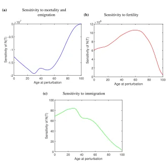
Figure 1 shows the sensitivity of the total population sizeN(T), at terminal timeT = 40, to changes in the vital rates applied in every projection year, as a function of the age at which the vital rate is perturbed, as shown in equations (49) and (51).
Figure 1: Sensitivity of total population size
(a) Sensitivity to mortality and emigration
Age at perturbation
0 20 40 60 80 100
Sensitivity of N(T)
×107
-2 -1.5 -1 -0.5 0
(b) Sensitivity to fertility
Age at perturbation
0 20 40 60 80 100
Sensitivity of N(T)
×106
0 2 4 6 8 10 12
(c) Sensitivity to immigration
Age at perturbation
0 20 40 60 80 100
Sensitivity of N(T)
0 20 40 60 80 100
Notes: The sensitivity of the total population sizeN(T), at the terminal timeT= 40, to changes in age-specific vital rates, applied in every year fromt= 0tot=T. (a) Sensitivity to age-specific mortality or emigration, which are indistinguishable in this model. (b) Sensitivity to age-specific fertility, (c) Sensitivity to age-specific immigration. Based on Instituto Nacional de Estad´ıstica (2012c) projections for Spain from 2012 to 2052.
cohorts pass through age groups 30 to 40 at the beginning of the projection period, so that any perturbations in the vital rates concern large population numbers. The effects of perturbations also accumulate during the projection period, as population members move to older age groups.
Additive perturbations in either mortality or emigration rates have a w-shaped effect onN(T), with effects being largest around age 30 and to a lesser extent around age 50. Increasing rates at these ages by one unit during the projection period would reduce the final population size by between1.8×107and2×107units. Perturbations at other ages,
especially above age 65, would have a smaller effect on the final population size. Perturbations in immigration also have the strongest effect on the final population size if they occur at young adult ages. At age 30, increasing immigration numbers by one unit, i.e. by one male and one female immigrant per projection year, increases the final population size by more than 80 persons. This includes the additional immigrants them-selves and their offspring. At ages above 30, the effect of perturbations in immigration numbers decreases. The sensitivities to changes in immigration are many orders of mag-nitude smaller than those to changes in the other vital rates. This is because immigration is measured in numbers, while mortality/emigration and fertility are per capita rates. As we will see below, elasticities help such comparisons by scaling values as proportional perturbations.
The sensitivity of total population size to perturbations in fertility rates increases with age. INE has defined fertility assumptions for women of ages 15 to 49. Among these age groups, perturbations at age 49 have the strongest effect on the total population size at timeT = 40. An increase in fertility rates by one unit across all projection years would increase the final population size by around10×106units. Figure 1 also shows that
perturbations in fertility at higher ages would have even larger effects. Unless women’s fertility could be extended beyond age 50 in the future, this result is only of theoretical interest.
5.2 Elasticity of male and female population sizes
While Figure 1 compares the effects of additive perturbations across ages, comparisons between vital rates are difficult, because immigration assumptions are defined in terms of numbers and fertility and mortality/emigration assumptions as rates. In order to compare the effect of perturbations across vital rates, we calculate elasticities. Figure 2 shows the elasticity of the male and female populations atT = 40to perturbations in mortality, fertility and migration as a function of the ages at which perturbations occur.
immi-gration numbers and emiimmi-gration rates. If the female population increases, this increases the number of male offspring. The female population, by contrast, is not directly affected by perturbations in male migration. For similar reasons, the male population reacts more strongly to perturbations in fertility than the female population. The elasticity of the final male and female population sizes to perturbations in fertility is highest around age 35. The elasticity results thus confirm that projection parameters at ages 25 to 35 have to be defined with particular care if the projection outcome of interest is the final population size.
Figure 2: Elasticity of male and female population sizes
(a) Male population
Age at perturbation
0 20 40 60 80 100
Elasticity of male population
-0.015 -0.01 -0.005 0 0.005 0.01 0.015 0.02
Mortality Fertility Immigration Emigration
(b) Female population
Age at perturbation
0 20 40 60 80 100
Elasticity of female population
-0.015 -0.01 -0.005 0 0.005 0.01 0.015 0.02
Mortality Fertility Immigration Emigration
Notes: The elasticity of total male and female population sizeN(T), at the terminal timeT= 40, to changes in age-specific vital rates, applied in every year fromt= 0tot=T. (a) Elasticity of the total male population, (b) Elasticity of the total female population. Based on Instituto Nacional de Estad´ıstica (2012c) projections for Spain from 2012 to 2052.
Population size is most affected by changes in mortality in old age — around 85 years for males and 90 years for females. Because mortality is low at early ages, pro-portional changes have little impact and the aging population increases the importance of changes affecting old individuals.
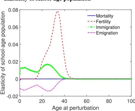
5.3 Elasticity of the school-age population (6 to 16 years)
Again, we focus on the size of this population group atT = 40and assume that pertur-bations have occurred throughout the projection period.
Figure 3: Elasticity of school-age population
Age at perturbation
0 20 40 60 80 100
Elasticity of school-age population
-0.02 0 0.02 0.04 0.06 0.08
Mortality Fertility Immigration Emigration
Notes: The elasticity of the school-age population size (6–16 years), at the terminal timeT= 40, to changes in age-specific vital rates, applied in every year fromt= 0tot=T. Based on Instituto Nacional de Estad´ıstica (2012c) projections for Spain from 2012 to 2052.
5.4 Elasticity of population with dementia
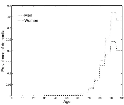
It is often interesting to project the health status of a population. Here, we weight the population by the age-specific prevalence of dementia (Alzheimer Europe 2014) and cal-culate the elasticity of the number of persons with dementia atT = 40to perturbations in the vital rates and in the prevalence schedule. Figure 4 shows the prevalence of dementia by age among the Spanish population in 2012. Prevalence increases strongly above age 70, and is higher for women than for men. We use these prevalences as the weight vector cin (35). Figure 5 shows the elasticity of the projected population with dementia in 2052 (male and female cases combined) to perturbations.8
Figure 4: Prevalence of dementia in Spain, 2012
0 10 20 30 40 50 60 70 80 90 100 0
0.05 0.1 0.15 0.2 0.25 0.3 0.35 0.4
Age
Prevalence of dementia
Men Women
Notes: (Age- and sex-specific prevalence of dementia in Spain in the year 2012 from Alzheimer Europe (2014).
The number of persons with dementia reacts most strongly to perturbations in the prevalence schedule. A one percent increase at any age between 85 and 90 years across projection years, for instance, would increase the number of dementia cases in the last projection year by between 0.05 and 0.06 per cent. Perturbations in the vital rates have smaller effects. Changes in mortality and migration before age 30 have no effect because persons in these age groups are rarely susceptible to dementia before the end of the pro-jection. For the same reason, changes in fertility have no effect. Above age 30, the effect
8We project the future number of dementia cases by holding current prevalence rates constant. For a similar
of perturbations in mortality, emigration and immigration increases, reaching its highest level at ages 55 (emigration) and 60 (immigration). Perturbations of mortality show the largest impact between ages 85 and 90, when prevalence rates in dementia reach high levels. Overall, however, developments in the prevalence of dementia appear to be more decisive for the future number of dementia cases than trends in the vital rates.
Figure 5: Elasticity of the population with dementia
Age at perturbation
0 20 40 60 80 100
Elasticity of dementia population
-0.04 -0.02 0 0.02 0.04 0.06
Mortality Fertility Immigration Emigration
Dementia prevalences
Notes: Elasticity of the population with dementia at the terminal timeT= 40to changes in age-specific vital rates and prevalences, applied in every projection year fromt= 0tot=T. Based on Instituto Nacional de Estad´ıstica (2012c) projections for Spain from 2012 to 2052 and dementia prevalence from Alzheimer Europe (2014).
5.5 Elasticity of dependency and support ratios
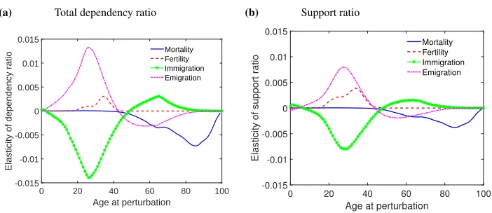
One of the findings highlighted by INE is that the dependency ratio (defining persons under age 16 and over age 64 as dependent) will double during the projection period. In 2052, the dependent population is expected to be as large as the population of working age. We show the elasticities of the dependency ratio atT = 40, calculated from (39) and (40), in Figure 6.
The elasticity to the mortality rate increases above age 40 and reaches a maximum around age 85. Perturbations in fertility rates have the proportionally smallest effect. This is because during the 40-year projection period, newborn cohorts contribute both to the size of age groups defined as dependent and to the working age population, and the effects cancel each other out to some extent.
Figure 6: Elasticity of dependency and support ratio
(a) Total dependency ratio
Age at perturbation
0 20 40 60 80 100
Elasticity of dependency ratio
-0.015 -0.01 -0.005 0 0.005 0.01 0.015
Mortality Fertility Immigration Emigration
(b) Support ratio
Age at perturbation
0 20 40 60 80 100
Elasticity of support ratio
-0.015 -0.01 -0.005 0 0.005 0.01 0.015
Mortality Fertility Immigration Emigration
Notes: The elasticity of the total dependency ratio and the economic support ratio at the terminal timeT= 40to changes in age-specific mortality, fertility, and migration, applied in every year fromt= 0tot=T. (a) Elasticity of the total dependency ratio (dependent ages: below age 16 and above age 64), (b) Elasticity of the economic support ratio. The signs of these elasticities are reversed to make the figure comparable to the elasticities of the dependency ratio; see text for details. Based on Instituto Nacional de Estad´ıstica (2012c) projections for Spain from 2012 to 2052 and age-specific consumption and labour income data from the National Transfer Accounts Project: http://ntaccounts.org
The dependency ratio used by INE is a simplified description of economic depen-dency. It disregards individuals above age 65 who continue to be productive and those 16–64 who are not part of the labour force. A more nuanced perspective is provided by the economic support ratio (Prskawetz and Sambt 2014), which is the ratio of total labor income to total consumption. These ratios can be calculated from age-specific income and consumption data prepared by the National Transfer Accounts (NTA) Project.9 We calculated support ratios for Spain, based on these NTA data for the year 2000, using per capita normalised annual consumption (public and private consumption) and labour income flows as weight vectors, as in (39).
Figure 6 shows the elasticities of the support ratio atT = 40to perturbations in the vital rates, applied in every projection year.10 The elasticities of the two indices are
similar, but less pronounced, except for the elasticity to fertility. Increases in fertility have a larger effect on the support ratio. This reflects Spanish income and consumption patterns in 2000, in which consumption is greater than income until about age 24. Young persons therefore remain ‘net consumers’ for longer than assumed by the dependency ratio, and the net effect of increases in fertility would be to put a downward pressure on the support ratio.
6. Discussion
6.1 Sensitivity analysis and scenarios
Population projections are hungry for demographic data. The projection of Spain, in which 101 ages are projected over 40 years on the basis of annual rates of mortality, fertility, immigration, and emigration, contains over 16,000 pieces of information. The result of all this information is a diverse set of outcomes: population vectors, population sizes (weighted in various ways), population ratios, growth rates, etc. Changes in any of the parameters at any time will change these results. The sensitivity structure quantifies these effects.
Disciplines in which sensitivity analyses of various kinds have become common (e.g., population ecology from the 1980s onwards) experience a shift in perspective, in which the sensitivity of a dependent variable becomes as much a part of the analytical results as the dependent variable itself. From this perspective, until you have analyzed the sensitivity relationships, you have not understood the model.
Statistical offices and agencies often repeat their projections under multiple scenar-ios (low, medium, high, etc.). Such scenario-building is a kind of perturbation analysis, quantifying the effects of large changes imposed on many vital rates simultaneously, but the number of possible scenarios is effectively infinite. In contrast, sensitivity and elas-ticity analyses provide a quantitative measure of the effects of perturbations of specific rates. For example, from graphs like Figures 5 and 6, we know, without the need for any scenario modifications at all, that given changes in the vital rates would have smaller ef-fects on the number of persons with dementia than would changes in the prevalence rates. We know that changes in fertility will have different effects on the economic support ra-tio than on the total dependency rara-tio. Such conclusions may help decide what kind of scenario modifications are most worth examining.
6.2 Sensitivity and uncertainty
Because population projections are used for social, economic, and ecological planning, demographers have invested considerable attention to measuring their uncertainty. A large body of literature has focused on probabilistic population projections based on past projection errors, expert opinion or stochastic models (Keilman, Pham, and Hetland 2002).
Sensitivity analysis does not, by itself, provide information on the uncertainty of a projection [it is a prospective, not a retrospective, perturbation analysis, in the termi-nology of Caswell (2000)]. Knowing that an outcome is more or less sensitive to some parameter does not tell whether the outcome is more or less certain. That also depends on the precision with which the parameter is estimated.
When this precision is known, sensitivity analysis provides a powerful way to trans-late it into the uncertainty in projection outcomes. Suppose thatξis a projection result (vector- or scalar-valued) that depends on a set of parametersθ. The uncertainty in the estimate ofξis measured by the covariance matrix
C(ξ) = Cov(ξi,ξj) . (57)
Ifξis a scalar, this is simply the varianceV(ξ).
The uncertainty in the parameter estimates is quantified by the covariance matrix C(θ), which might be obtained, e.g., from the Fisher information matrix provided by maximum likelihood estimation ofθ.
Then, to first order, the uncertainty inθtranslates into uncertainty inξby
C(ξ) = dξ dθT C(θ)
dξ
dθT T
. (58)
Ifξis a scalar, this reduces to
V(ξ) = dξ dθT C(θ)
dξ
dθT T
(59)
and ifθis also a scalar, then
V(ξ) =
dξ
dθ 2
V(θ). (60)
6.3 Immigration and emigration
Migration is challenging to model. Births, deaths, and emigration are events that happen to individuals in the population under study. They can be described by rates, estimated from the number of events and the number of individuals at risk. Those rates can be transformed to probabilities and then applied to the appropriate components of cohorts to project the population forward.
Immigration, however, is not an event to which individuals in the population are at risk, and hence it cannot be described as a rate. Thus, in equations (4), (7), and (8), immigration appears as a vectorb(t), with units of numbers of individuals, rather than as one of the per capita rates inUandF.
Immigration is handled in various ways by the agencies engaged in projections. The projection of Spain in Section 4 takes the sensible approach of separating emigration and immigration, including emigration along with mortality in the matrixU, and placing immigration inb(t). The projections prepared by Eurostat (Lanzieri 2009) make this approach slightly more subtle, noting that individuals who immigrate during(t,t+ 1)
spend some fraction of the interval in the population, and hence subject to the mortality and fertility rates in action during that time (G. Lanzieri, personal communication). This means that a basic projection equation becomes
n(t+ 1) =A(t)n(t) +B(t)b(t) (61)
whereB(t) is a matrix that includes mortality and fertility of immigrants during the fraction of the interval during which they are assumed to be present (usually 0.5 years). Our approach is easily extended to the projection (61), for example, simply by replacing the termdb(t)/dθT(s)in equation (13) with
B(t)db(t) dθT(s)+
bT(t)⊗I ω
dvecB(t) dθT(s) .
A different approach defines the additive vectorbasnetmigration (immigration−
emigration), thus treating both immigration and emigration as additive. This has unfortu-nate theoretical properties; it asserts that the number of individuals leaving the population is independent of the population at risk of leaving. In principle, in the long run this could draw a population down to impossible negative values. For the short time horizons in practical population projections, this is unlikely to be a problem.
These models focus on a single population. The analysis of migration can also be embedded in a multiregional model (Rogers 1975), in which the immigrants to one pop-ulation come from the emigrants leaving another poppop-ulation. Such multiregional models are a special case of multistate models (Rogers 1985) and the beginnings of the theory for sensitivity analysis of multistate models exists (Caswell 2012; Caswell and Salguero-Gomez 2013). We will explore the sensitivity analysis of multistate projections in a subsequent paper.
All of these approaches produce linear projections that are simple modifications of the basic models (4)–(8). There is also a tradition of theories that model migration as a function of population size, distance, and other properties of origin and destination. These models are descendants of the Zipf (1946) gravity model. Courgeau (1995) discusses how these models arise from theories of choice. They lead to expressions in which the log of the number of migrants from locationito locationj is a linear function of the logs of population size, distance, and other variables. Cohen et al. (2008) and Kim and Cohen (2010) have applied the method in a detailed analysis of data on international migration and were able to capture significant amounts of the variance in migration flows.
Because migration in gravity models is a power function of population size, the resulting projections are nonlinear. We do not address the analysis here, but note that sensitivity analysis can also be applied to nonlinear models (Caswell 2007, 2008), a de-velopment noted by Cohen et al. (2008) as an open research question.
6.4 Data requirements and applications
Goldstein and Stecklov (2002) have lamented the lack of clarity and transparency in re-ports of population projections. The trajectories of mortality, fertility, and immigration on which the projections depend are seldom reported, and “even when extensive documen-tation is provided, it is difficult to replicate the calculations without access to proprietary computer software used by the team that prepared the projection” (Goldstein and Stecklov 2002, p. 121). We urge agencies to consider reporting the basis of their projections in the form of projection matrices. The entries ofU,F, andbmay require considerable effort to obtain, and sophisticated methods may be needed to estimate them from data on pop-ulations, births, deaths, etc. But once the estimation process is completed, the projection matrix formulation provides a readily computable, non-proprietary method of studying the results and exploring scenarios. The mathematical relationships extracted from those matrices will be valid regardless of how the matrices themselves are obtained. Sensitivity analysis is just one of their possible uses.
sensitivity and elasticity analyses can be extended to multistate population projections; these developments are left for future research. In the meantime, the analyses presented here will benefit demographers and government officials producing projections, because they will improve our understanding of the underlying mechanisms leading to uncertain-ties and allow for precise quantifications of the impact of changes in vital rates or policies on any projection output.
7. Acknowledgements
References
Abadir, K.M. and Magnus, J.R. (2005). Matrix algebra. New York: Cambridge Univer-sity Press.
Ahlburg, D. and Lutz, W. (1998). Introduction: The need to rethink approaches to pop-ulation forecasts. Population and Development Review 24(Supplement. Frontiers of Population Forecasting): 1–14. doi:10.2307/2808048.
Alzheimer Europe (2014). The prevalence of Dementia in Europe http://www.alzheimer- europe.org/Policy-in-Practice2/Country-comparisons/The-prevalence-of-dementia-in-Europe.
Arthur, W.B. (1984). The analysis of linkages in demographic theroy.Demography21(1): 109–128.doi:10.2307/2061031.
Booth, H. (2006). Demographic forecasting: 1980 to 2005 in review. International Journal of Forecasting22(3): 547–581. doi:10.1016/j.ijforecast.2006.04.001.
Caswell, H. (2000). Prospective and retrospective perturbation analyses: Their roles in conservation biology. Ecology81: 619–627.doi:10.2307/177364.
Caswell, H. (2001). Matrix Population Models: Construction, Analysis, and Interpreta-tion. Sunderland: Sinauer Associates, second ed.
Caswell, H. (2006). Applications of Markov Chains in Demography. In: Langville, A.N. and Stewart, W.J. (eds.).MAM2006: Markov Anniversary Meeting. Raleigh: Boson Books: 319–334.
Caswell, H. (2007). Sensitivity analysis of transient population dynamics. Ecology Let-ters10(1): 1–15.doi:10.1111/j.1461-0248.2006.01001.x.
Caswell, H. (2008). Perturbation analysis of nonlinear matrix population models. Demo-graphic Research18: 59–116.doi:10.4054/DemRes.2008.18.3.
Caswell, H. (2009). Stage, age, and individual stochasticity in demography. Oikos
118(12): 1763–1782.doi:10.1111/j.1600-0706.2009.17620.x.
Caswell, H. (2010). Reproductive value, the stable age distribution, and the sensitivity of the population growth rate to changes in vital rates. Demographic Research 23: 531–548.doi:10.4054/DemRes.2010.23.19.
Caswell, H. (2012). Matrix models and sensitivity analysis of populations classified by age and stage: A vec-permutation matrix approach. Theoretical Ecology5(3): 403–
417. doi:10.1007/s12080-011-0132-2.
Jour-nal of Ecology101(3): 585–595.doi:10.1111/1365-2745.12088.
Caswell, H. and Shyu, E. (2012). Sensitivity analysis of periodic matrix population mod-els. Theoretical Population Biology82(4): 329–339.doi:10.1016/j.tpb.2012.03.008.
Cohen, J.E., Roig, M., Reuman, D.C., and GoGwilt, C. (2008). International migration beyond gravity: A statistical model for use in population projec-tions. Proceedings of the National Academy of Sciences 105(4): 15269–15274.
doi:10.1073/pnas.0808185105.
Colantuoni, E., Surplus, G., Hackman, A., Arrighi, H.M., and Brookmeyer, R. (2010). Web-based application to project the burden of Alzheimer’s disease. Alzheimer’s and Dementia6(5): 425–428.doi:10.1016/j.jalz.2010.01.014.
Courgeau, D. (1995). Migration theories and behavioural models. International Journal of Population Geography1(1): 19–27.doi:10.1002/ijpg.6060010103.
Ekamper, P. and Keilman, N. (1993). Sensitivity analysis in a multidimensional demo-graphic projection model with a two-sex algorithm. Mathematical Population Studies
4(1): 21–36.doi:10.1080/08898489309525354.
Engelman, M., Caswell, H., and Agree, E. (2014). Why do lifespan variability trends for the young and old diverge? A perturbation analysis. Demographic Research30: 1367–1396.doi:10.4054/DemRes.2014.30.48.
Fox, P.J., Kohatsu, N., Max, W., and Arnsberger, P. (2001). Estimating the costs of caring for people with Alzheimer Disease in California: 2000-2040.Journal of Public Health Policy22(1): 88–97.doi:10.2307/3343555.
Gerland, P., Raftery, A., Sevcikova, H., Li, N., Gu, D., Spoorenberg, T., Alkema, L., Fosdick, B., Chunn, J., Lalic, N., Bay, G., Buettner, T., Heilig, G., and Wilmoth, J. (2014). World population stabilization unlikely this century. Science346(6206): 234– 237.doi:10.1126/science.1257469.
Goldstein, J.R. and Stecklov, G. (2002). Long-range population projections made sim-ple. Population and Development Review 28(1): 121–141.
doi:10.1111/j.1728-4457.2002.00121.x.
Hunter, C.M., Caswell, H., Runge, M.C., Regehr, E.V., Amstrup, S.C., and Stirling, I. (2010). Climate change threatens polar bear populations: a stochastic demographic analysis.Ecology91(10): 2883–2897.doi:10.1890/09-1641.1.
Instituto Nacional de Estad´ıstica (2012a). Press Release. Population projections for 2012 http://www.ine.es/en/prensa/np744 en.pdf.
Instituto Nacional de Estad´ıstica (2012c). Demographic evolution parameters 2012–2051
http://www.ine.es/jaxi/menu.do?type=pcaxis&path=%2Ft20%
2Fp251&file=inebase&L=1.
Jenouvrier, S., Caswell, H., Barbraud, C., Holland, M., Stroeve, J., and Weimerskirch, H. (2009). Demographic models and IPCC climate projections predict the decline of an emperor penguin population.Proceedings of the National Academy of Sciences106(6): 1844–1847.doi:10.1073/pnas.0806638106.
Jenouvrier, S., Holland, M., Stroeve, J., Barbraud, C., Weimerskirch, H., Serreze, M., and Caswell, H. (2012). Effects of climate change on an emperor penguin population: analysis of coupled demographic and climate models. Global Change Biology18(9): 2756–2770.doi:10.1111/j.1365-2486.2012.02744.x.
Jenouvrier, S., Holland, M., Stroeve, J., Serreze, M., Barbraud, C., Weimerskirch, H., and Caswell, H. (2014). Projected continent-wide declines of the emperor penguin under climate change.Nature Climate Change4: 715–718. doi:10.1038/nclimate2280.
Keilman, N., Pham, D.Q., and Hetland, A. (2002). Why population forecasts should be probabilistic – illustrated by the case of Norway. Demographic Research6: 409–454.
doi:10.4054/DemRes.2002.6.15.
Keyfitz, N. (1964). The population projection as a matrix operator. Demography1(1): 56–73.doi:10.1007/BF03208445.
Kim, K. and Cohen, J.E. (2010). Determinants of international migration flows to and from industrialized countries: A panel data approach beyond gravity. International Migration Review44(4): 899–932.doi:10.1111/j.1747-7379.2010.00830.x.
Lanzieri, G. (2009). Europop2008: A set of population projections for the European Union. Paper presented at XXVI IUSSP International Population Conference, Mar-rakech, Morocco, September 27 – October 02 2009.
Magnus, J.R. and Neudecker, H. (1985). Matrix differential calculus with applications to simple, Hadamard, and Kronecker products. Journal of Mathematical Psychology
29(4): 474–492. doi:10.1016/0022-2496(85)90006-9.
Magnus, J.R. and Neudecker, H. (1988).Matrix differential calculus with applications in statistics and econometrics. New York: John Wiley and Sons.
Prskawetz, A. and Sambt, J. (2014). Economic support ratios and the
de-mographic dividend in Europe. Demographic Research 30: 963–1010.
doi:10.4054/DemRes.2014.30.34.
Rogers, A. (1985).Regional population projection models. Beverly Hills: Sage.
Roth, W.E. (1934). On direct product matrices. Bulletin of the American Mathematical Society40: 461–468.doi:10.1090/S0002-9904-1934-05899-3.
Samuelson, P.A. (1947). Foundations of economic analysis. Cambridge, MA: Harvard University Press.
van Raalte, A. and Caswell, H. (2013). Perturbation analysis of indices of lifespan vari-ability.Demography50(5): 1615–1640.doi:10.1007/s13524-013-0223-3.
Wancata, J., Musalek, M., Alexandrowicz, R., and Krautgartner, M. (2003). Number of Dementia sufferers in Europe between the years 2000 and 2050.European Psychiatry
18(6): 306–313. doi:10.1016/j.eurpsy.2003.03.003.
Willekens, F.J. (1977). Sensitivity analysis in multiregional demographic models. Envi-ronment and Planning A9(6): 653–674.doi:10.1068/a090653.
Zipf, G..K. (1946). The p1p2/d hypothesis: On the inter-city movement of persons.