An Algorithm for the Estimation of the Initial Text Skew

An Algorithm for the Estimation of the Initial Text Skew

Darko Brodi

ć

, Dragan R. Milivojevi

ć

V.J. 12, 19210 Bor, Serbia e-mail: [email protected]

2 _{Mining and Metallurgy Institute, Department of Informatics,}

Z. Bulevar bb, 19210 Bor, Serbia e-mail: [email protected]

http://dx.doi.org/10.5755/j01.itc.41.3.1249

Abstract. The paper presents a methodology for the estimation of the initial skew rate of text lines. Firstly, it splits text into groups according to the bounding boxes. Linked bounding boxes establish the bigger objects called connected components. After applying mathematical morphology operations, the enlarged group of the connected components is formed. The longest connected component is extracted by the longest common subsequence method. Inside the longest connected component, the gravity centers are determined for each bounding box. They represent the reference points, which are used for the calculation of the initial skew rate. Calculation is made by the moment based method. The comparative analysis of the origin and estimated skew rate is used to evaluate the algorithm. Hence, the proposed algorithm is examined withdifferent printed text samples. It showed robustness for the skew estimation in the wide range of resolutions.

Keywords: Document image processing; Text skew; Initial text skew; Moments; Printed text.

1. Introduction

The old documents have been saved mainly in the printed form. Those documents have to be converted from the printed to electronic form. This process is done by scanning. However, the obtained electronic form is not completely editable. Hence, the main role is the transformation of the document image into a computer editable form. For this purpose, the optical character recognition (OCR) system is used. If in document image the skew exists, then OCR will fail. Hence, the skew makes this process more complex. That’s why the skew identification has an important role in the preprocessing stage of the OCR [1].

Printed text represents a pretty well formed text type. It has a strong regularity in shape, which is characterized with the uniform skewness. Decent spacing between nearby text lines with descendant and ascendant characters enables the constant separation of them. Hence, the distance between them is a quite sufficient. At the end, the printed text is considered as a predictable one.

The known methods for the skew estimation are classified as follows [1]: Histogram analysis method, K-nearest neighbor clustering method, Cross-correlation method, Hough transforms method, Fourier transformation method, and other methods.

Histogram analysis represents the widely used method for the skew estimation in printed text. It is based on the identification of the minima in the horizontal pixel density histogram [2]. However, this method is suited for the uniform skew only. Hence, it failed to identify the skew in column or multi-line text.

K-nearest neighbor clustering method is based on the page layout analysis [3]. This method forms the connected components by nearest neighbors clustering, which represents the characters themselves. Still, it is characterized with the poor text line segmentation. Hence, its application is suitable primarily for Roman languages.

The cross-correlation method calculates the similarity between the original (document text) and referent image. It forms the histogram of cross-correlation. Furthermore, it compares the shift of the interline cross-correlation to determine the skew rate. However, the method is suited for small skew angles up to 10° [4].

image domain. If scattered text is under consideration, then the difficulties in choosing a peak in Hough space are one of major limitation of the method. In addition, the method is complex and computer time intensive.

The Fourier transform method is a Fourier domain representation of the projected profile method in the pixel domain. This way, it is just a similar methodology as projected profile, but in different domains [6].

The techniques classified as other methods are based mostly on geometrical transformation. These algorithms are typically computationally inexpensive.

The simplest method based on the polygon gravity centers for skew estimation has been proposed in [7]. The simplicity and global approach represent its advantage. However, its accuracy is lower than 87%.

Another method based on boundary growing approach is proposed in [8]. It is a simple and computationally inexpensive method. However, it contains few constraints based on text elements pre assumptions. Hence, the modified method, which solves some of these disadvantages, is given in [9]. Compared with other methods, the obtained results are promising.

The paper describes a modification of the method based on the bounding boxes, and theirs gravity center points [9]. The initial method is extended with the binary dilatation. It creates the connected component objects. Further, the longest connected component is selected. In addition, some constraints of the original algorithm have been overcome. The proposed algorithm shows the skew estimation accuracy of the document images in standard and low resolutions. Hence, it is characterized as robust method.

Organization of this paper is following. Section 2 describes the proposed algorithm. Section 3 defines text experiments. Section 4 compares and discusses the results. Section 5 makes conclusions.

2. The algorithm

Digital document text image is a product of the image scanning. It is a digital gray-level image, which is represented by matrix D. It consists of M rows, N columns, and contains the elements whose intensity has L discrete levels of gray. L is the integer from {0, …, 255}, D(i, j)  {0, …, 255}, where i = 1, …, M and j = 1, …, N. After performing the binarization procedure the image represented by matrix D is transformed into binary image B(i, j). Its entries are equal to 1 if D(i, j) ≥ Dth(i, j), or to 0 if

D(i, j) < Dth(i, j), where Dth is given by any local

binarization method [10-11]. Dth represents local

threshold sensitivity decision value. Currently, document image is given as binary matrix B featuring M rows and N columns.

In the original algorithm [8-9], the key assumption was that spacing of adjoining text lines is always sufficient. However, this premise was the main constraint in the real circumstances. Hence, to

overcome that condition, the new elements in the algorithm are proposed. The algorithm consists of six steps as follows:

1. Extraction of the bounding boxes, 2. Morphological dilatation,

3. Longest connected components extraction, 4. Gravity centers determination,

5. Reference text line estimation, 6. Document image rotation.

Step 1. Extraction of the bounding boxes.

The bounding box represents a rectangular region whose edges are parallel to the coordinate axes [12]:

) (

) (

| ) ,

(i j i_min i i_max j_min j j_max

X      , (1)

where imax, imin, jmax, and jmin represent the endpoints of

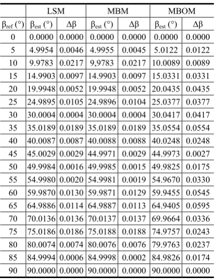
the bounding box. The algorithm creates a bounding box around each text object, which is primarily character. Then, each bounding box is filled with black pixels. Furthermore, all associated filled bounding boxes establish the object called connected component. They create a new image with connected components represented by binary matrix Y. It is shown in Figure 1(b).

(a)

(b)

Figure 1. Document text image and its counterpart with connected components: (a) Matrix B, (b) Matrix Y

Step 2. Morphological dilatation.

To separate every text line, each connected component is growing in all directions. It is accomplished with morphological dilatation applied to

Y. This way, the adjacent connected components are merged establishing the text line. This process facilitates text line segmentation, but may lead to joining and merging nearby text lines. Assumption that text line spacing is always sufficient was the main constraint of the original algorithm [8-9]. In ourcase,

200 400 600 800 1000 1200 1400 1600 1800 2000 2200 200

the bounding boxes are not growing in all directions to the nearby bounding box of the next character. Thus, the main assumption on sufficient text line spacing is superfluous. To overcome it, printed text characteristics should be examined. Definition of the typical printed text leading i.e. line spacing is given in Figure 2.

Figure 2. Definition of the typical printed text leading

Interline spacing represents 20% of text point size [13]. This information is crucial for overcoming the original algorithm’s disadvantage done by the pre-assumption. For morphological dilatation, the structuring element Ln with variable width line

accompanying allowed interline spacing is used. Morphological operation is given as:

n  n

Z Y L , (2)

where n = 1, ..., U, and U = 3. It means that three variable width lines are used. Experiment shows that the number of structuring elements higher than 3 is unnecessary [13].

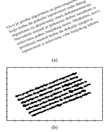
Step 3. Longest connected components extraction. From Zn the longest connected components CCLNG

can be extracted with the longest common subsequence (LCS) (See Appendix) [13]. It is obtained as follows:



, 1

max U ( , )

LNG n i j n

CC Z i j



 

 _{ }





The longest connected component CCLNG is shown

in Figure 3.

Figure 3. The extracted longest connected component

CCLNG

Step 4. Gravity centers determination.

The longest connected component CCLNG is

compiled from the filled bounding boxes BBK.

Accordingly, K = 1 …, Q, where Q represents the number of bounding boxes that form the longest connected component. Each of the bounding boxes has its own gravity center represented with a gravity center pixel GC. The coordinates of this pixel are determined by the bounding box endpoints imax, imin,

jmax, and jmin. Hence, the gravity center pixel is given

as:

LNG

min, max, min, max,

, ₂ , ₂

K K K K

CC K

i i j j

GC _{ }   _

 . (4)

This is illustrated in Figure 4.

(a)

(b)

Figure 4. Gravity centers of the longest connected component: (a) each intersection represents the gravity

center, (b) gravity centers of each bounding box

Set of these Q pixels is the cornerstone for the calculation of the reference line of the longest connected component, which is characterized as initial skew of the printed text. This value of skew is very closeto the estimated printed text skew.

Step 5. Reference text line estimation.

Reference text line in printed text is linear. It can be estimated with different calculation method. In this paper, the least square method (LSM) and moment based method (MBM) are used.

(a) Least square method (LSM). The first-degree polynomial function approximation is given as:

lsm lsm

y a x b  , (5)

where alsm is the slope and blsm is y-intercept.

Furthermore, the slope alsm, and y-intercept blsm are

calculated as [8,14]:

LNG LNG LNG LNG

LNG LNG

, , , ,

1 1 1

2 2

, ,

1 1

Q Q Q

CC K CC K CC K CC K

K K K

lsm _{Q Q}

CC K CC K

K K

Q x y x y

a

Q x x

  

 

   

  _{  } _

   



 

 _{  }

 











,(6)

and

LNG, , LNG

1 1

Q Q

CC K lsm CC K

K K

lsm

y a x

b

Q

 

 







where Q is the number of data in the set. Hence, the initial text skew angle for the longest connected components is defined as:

arctan( )

lsm alsm

  . (8)

(b) Moment based method (MBM). Moment defines the measure of the pixel distribution in the image. It identifies global image information concerning its

200 400 600 800 1000 1200 1400 1600 1800 2000 2200 200

contour. The (p+q)-th order geometric moment mpq of

a gray-level image D is defined as:

1 1

( , )

N M p q pq

i j

m i j D i j

 



_{ }

In eq. (9) p and q = 0, 1, 2, 3, ..., n, and n represent the order of the moment. Accordingly, for the binary image B geometric moment’s mpq are defined as

[15-16]:

1 1

N M p q pq

i j

m i j

 





From eq. (10) central moment’s μpq for the binary

image B can be calculated as:

1 1

( ) ( )

N M

p q

pq i j

i x j y



 



_

In eq. (11) xand yrepresent the coordinates of the centre of mass, i.e. gravity center (GC), which are given as:

10 01

00 00

,

m m

x y

m m

  , (12)

where m00 is the area of the object in binary image B.

Some of the important image features can be obtained from the moments. The second order moments {μ02,

μ11, μ20} may be used to determine an image

orientation [15-16]. In general, the orientation of an image describes how the image lies in the field of view, or the directions of the principal axes. In terms of moments, the orientations of the principal axes are given by angle βMBM [15-16]:

11

20 02 2 1

arctan 2

MBM 



 

 

 _{ }



 

. (13)

Eq. (13) is valid for the skew estimation based on the gravity center points for the longest connected components. However, all these features represent the characteristics of the separate object, i.e. connected components. Therefore, this method can be used for the skew calculation of the longest connected component without extracting gravity center points. In this situation, we are dealing with derivation of the moment based method, which is called moment based object method (MBOM).

Step 6. Document image rotation. This step is illustrated in Figure 5.

(a)

(b)

Figure 5. Reference text line and skew determination: (a) Estimated reference text line, (b) Initial skew identification

needed for rotation

After obtaining estimated initial text skew, document text image has been rotated for that angle. Real text skew is close to the estimated initial text skew. However, a final adjustment is needed as well. It is made by repeating the described steps.

3. Experiments

3.1. Common measures

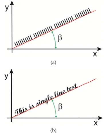
For the experiment, printed text sample, which is rotated up to 90° by step of 5° around x-axis, is used. This is illustrated in Figure 6.

(a)

(b)

Figure 6. Printed text sample rotated up to 90° in 5° steps: (a) Text sample 1, (b) Text sample 2

Their reference text line is given as:

y a x b   . (14)

The first evaluation measure is the absolute error. It is the difference between referent and estimated angle value:

ref est







 



200 400 600 800 1000 1200 1400 1600 1800 2000 2200 200

400 600 800 000 200 400 600 800



200 400 600 800 1000 1200 1400 1600 1800 2000 2200 200

400 600 800 1000 1200 1400 1600 1800

where ref is arctan of a given in eq. (14) whereas est

is given in eq. (8) and (13) respectively, for two different methods.

Furthermore, the evaluation measure of the reference line hit rate (RLHR) is introduced. It represents the algorithm succeed measure of retracing the original reference text line defined by [17-18]:

ref est ref RE

RLHR

  

   



1 ( ) 1 , (16)

where RE() represents a relative error of .

The third evaluation measure RMSE is calculated as [18]:

2

1

1

( )

R

k k ref est k

RMSE

R   





where k = 1, …, R and R is the number of the text samples.

4. Results and discussion

4.1. Single-line test

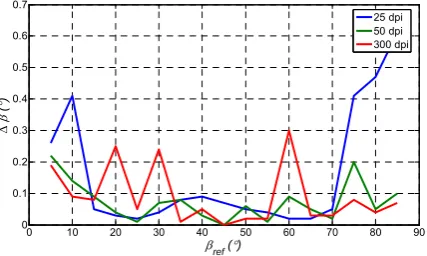
Firstly, the LSM (identical to MBM) algorithm is applied to the printed text sample in the whole angle range {0º, …, 90º}. The text sample 2 was in standard resolution of 300 dpi and in ultra low resolutions: 25 and 50 dpi. The obtained results are given in Table 1 (See Appendix). In this case, the algorithm without morphological dilatation has been applied. However, it is applied to the single text lineonly. This experiment is valid for the examination of the proposed algorithm’s accuracy. The results for the absolute error are shown in Figure 7.

Figure 7. Absolute error for the algorithm without dilatation (Text sample 2)

In the whole angle range, the absolute error is below 0.3° for the image in 300 dpi resolution. For the image in 50 dpi, the results are even better. Their absolute error is up to 0.2°. Reducing the resolution of the image to 25 dpi raises the absolute error up to 0.6°. Therefore, the error margin is small even for the ultra-low resolutions of the image. In addition, the image in ultra-low resolution of 50 dpi has been characterized with the smallest absolute error. In other words, the algorithm retraces the reference text line correctly.

RMSE values are calculated from the results given in Table 1 (See Appendix). These results are presented in Table 2 (See Appendix). The results for RMSE are also shown in Figure 8.

Figure 8. RMSE for the algorithm without dilatation (Text sample 2)

The small scattering of the results contributes to a small RMSE value. Therefore, these results just confirm above statements.

The results of the absolute error for the least square method (LSM), for the moment based method (MBM) and for the moment based object method (MBOM) are given in Table 3 (See Appendix). Their comparison for the text sample 1 in the resolution of 300 dpi is shown in Figure 9.

Figure 9. Absolute error for the algorithms: LSM, MBM and MBOM

In the whole angle range, the absolute error is below 0.02° for the LSM and MBM. In addition, their absolute error values are identical. LSM and MBM calculate the text skew by the gravity center points as the starting point. However, MBOM estimates the text skew by the moment based method which is applied to the object contour of the longest connected component only. Its absolute error is up to 0.06°. Although, it is a three times higher than LSM or MBM, this value is still rather small. It apparently seems that the relative values difference is significant, while in absolute terms it is negligible.

MBM and MBOM represent the moment-based methods. However, MBM calculates the text skew according to the moments of the gravity center points, while MBOM calculates the text skew according to the longest connected component contour. MBOM is slightly less accurate because of “the less accurate”

0 10 20 30 40 50 60 70 80 90

0 0.1 0.2 0.3 0.4 0.5 0.6 0.7

_ref ()





(



)

25 dpi 50 dpi 300 dpi

0 10 20 30 40 50 60 70 80 90

0.05 0.1 0.15 0.2 0.25 0.3 0.35 0.4

_ref ()

RM

S

E

25 dpi 50 dpi 300 dpi

0 10 20 30 40 50 60 70 80 90 0

0.01 0.02 0.03 0.04 0.05 0.06

_REF()



data inputs. This is a consequence of ascending and descending elements, which have a great impact on this method. However, MBOM is a less demanding procedure. The small number of steps that are needed for creating the input data for the algorithm proves that. The LSM or Hough transform (HT) have to exploit the set of gravity center points from the longest connected component for the text skew estimation. The moment-based method can use the same input data (MBM). However, it can use the contour of the longest connected component for the text skew estimation as well (MBOM). Therefore, the moment-based method has a clear advantage over LSM or even HT.

4.2. Multi-line test

In this experiment, the printed text samples consist of the rotated multi-line text in the whole range {0º, …, 90º}. However, the algorithm is extended by morphological dilatation. Furthermore, a new parameter is introduced. It represents the remaining number of the connected components CCALL. After

each dilatation, CCALL is decreasing. From the

remained number of CCALL, the longest one has been

extracted.

Aggregate test results are given in Table 4 (See Appendix). These results depend partly on the parameter CCALL.

The results for absolute error and RMSE are shown in Figures 10-11, respectively.

Figure 10. Absolute error in the algorithm extended by dilatation

Figure 11. Initial RMSE for the algorithm extended by dilatation

Estimation of the initial text skew is accurate in its whole tested range {0º, …, 80º}. However, it assertion is correct especially for the angles up to 65º (See Figure 10). Compared to the original algorithm [9-10], the results are much better in the wide-angle range. In addition, the algorithm does not depend on the column text type. Hence, it is suitable for a single as well as for the multi-column text. Furthermore, it can be recommended for the ultra-low resolution images, too. However, the proposed method is ready for use in printed text only. Still, the moment-based method applied to the object contour (MBOM) can be extended to the text type different from the printed one [19].

The method is characterized with the inferior results for the small angles. This is the consequence of the bounding boxes created by ascender and descender elements. Therefore, their gravity centers are considerably away from the typical initial text line. To overcome this disadvantage, the input data should be filtered by omitting the gravity centers of “large” bounding boxes for the calculation of the reference text line [20].

5. Conclusions

The paper describes the method for the skew estimation of the printed text based on the longest connected component. Firstly, it establishes the boundary growing area around text based on the filled bounding boxes. This way, the connected components have been created. The algorithm chooses the longest connected component by LCS method. Furthermore, the gravity centers of the bounding boxes are extracted. This set of points represents the input for the text skew estimation of the least square (LSM) and moment-based methods (MBM). Based on that, the initial text skew is estimated. Also, the initial skew rate is estimated from the longest connected component contour by the moment-based method (MBOM), too. Different methods are subjected to the single and multi-line text experiments. The experiment results confirm a low absolute deviation and good RMSE values in the tested angle range. Hence, all method proves theirs correctness for the estimation of the printed text skew. In addition, the extension of the algorithm with dilatation is examined. It is suitable for the multi-line and multi-column printed text without any segmentation. As an additional advantage, the extended method is computationally inexpensive. Due to its correctness, the method can be integrated partly or completely in the algorithms for the parameter extraction of the handwritten text. It is especially true for the moment-based object method. Future work should point out the efficient methodology for omitting the ascender and descender elements in bounding boxes of the longest connected component. It can be expected that these steps will further improve the accuracy of the initial skew rate method.

0 10 20 30 40 50 60 70 80

0 0.2 0.4 0.6 0.8 1 1.2 1.4 1.6 1.8

_ref ()





(



)

CC

ALL < 50

CC

ALL < 100

0 10 20 30 40 50 60 70 80

0.4 0.5 0.6 0.7 0.8 0.9 1

_ref ()

RM

S

E

CC

ALL < 50

CC

APPENDIX

Longest common subsequence (LCS) pseudo-code:

Longest objects from Z can be found out by so-called longest common subsequence (LCS) pseudo-code:

function LCSLength(A[1..M], B[1..N]) CC = array(1..M, 1..N)

for i := 1..M

CC[i,1] = 0

for j := 1..N

CC[1,j] = 0

for i := 1..M

for j := 1..N

if A[i] = B[j]

CC[i,j] := CC[i-1,j-1] + 1

else:

CC[i,j] := max(CC[i,j-1], CC[i-1,j])

return CC[m,n]

where matrix Z is defined by vectors A and B and resulted object is defined by matrix CC.

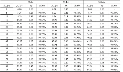
Table 1. Absolute error (Δβ) and RLHR for the bounding boxes gravity center algorithm (LSM or MBM – identical results) with the text sample 2 in different resolutions

25 dpi 50 dpi 300 dpi

βref (°) βest (°) Δβ RLHR βest (°) Δβ RLHR βest (°) Δβ RLHR

0 0.00 0.00 - 0.00 0.00 - 0.00 0.00 -

5 5.26 0.26 94.80% 5.22 0.22 95.60% 5.19 0.19 96.20%

10 9.59 0.41 95.90% 9.86 0.14 98.60% 9.91 0.09 99.10%

15 14.95 0.05 99.67% 14.91 0.09 99.40% 14.92 0.08 99.47%

20 19.97 0.03 99.85% 19.96 0.04 99.80% 19.75 0.25 98.75%

25 25.02 0.02 99.92% 24.99 0.01 99.96% 24.95 0.05 99.80%

30 29.96 0.04 99.87% 29.93 0.07 99.77% 29.76 0.24 99.20%

35 35.08 0.08 99.77% 35.08 0.08 99.77% 34.99 0.01 99.97%

40 40.09 0.09 99.78% 40.03 0.03 99.93% 40.05 0.05 99.88%

45 45.07 0.07 99.84% 45.00 0.00 100.00% 45.00 0.00 100.00%

50 49.95 0.05 99.90% 49.94 0.06 99.88% 49.98 0.02 99.96%

55 54.96 0.04 99.93% 54.99 0.01 99.98% 54.98 0.02 99.96%

60 59.98 0.02 99.97% 59.91 0.09 99.85% 59.70 0.30 99.50%

65 65.02 0.02 99.97% 64.95 0.05 99.92% 65.03 0.03 99.95%

70 70.05 0.05 99.93% 69.98 0.02 99.97% 69.97 0.03 99.96%

75 74.59 0.41 99.45% 74.80 0.20 99.73% 74.92 0.08 99.89%

80 79.53 0.47 99.41% 79.95 0.05 99.94% 79.96 0.04 99.95%

Table 2.RMSE for the algorithm (LSM or MBM – identical results) with the text sample 2 in different resolutions

RMSE βref (°) 25 dpi 50 dpi 300 dpi

0 - - -

5 0.2600 0.2200 0.1900

10 0.3433 0.1844 0.1487

15 0.2818 0.1593 0.1299

20 0.2445 0.1394 0.1682

25 0.2189 0.1247 0.1521

30 0.2005 0.1174 0.1699

35 0.1880 0.1128 0.1573

40 0.1787 0.1061 0.1482

45 0.1701 0.1000 0.1398

50 0.1622 0.0967 0.1327

55 0.1551 0.0923 0.1267

60 0.1486 0.0921 0.1491

65 0.1429 0.0896 0.1434

70 0.1383 0.0865 0.1385

75 0.1705 0.0982 0.1354

80 0.2026 0.0959 0.1314

85 0.2460 0.0962 0.1286

90 - - -

Table 3. Absolute error (Δβ) for the LSM, MBM and MBOM algorithm with the text sample 1 in 300 dpi

LSM MBM MBOM βref (°) βest (°) Δβ βest (°) Δβ βest (°) Δβ

0 0.0000 0.0000 0.0000 0.0000 0.0000 0.0000 5 4.9954 0.0046 4.9955 0.0045 5.0122 0.0122 10 9.9783 0.0217 9,9783 0.0217 10.0089 0.0089 15 14.9903 0.0097 14.9903 0.0097 15.0331 0.0331 20 19.9948 0.0052 19.9948 0.0052 20.0435 0.0435 25 24.9895 0.0105 24.9896 0.0104 25.0377 0.0377 30 30.0004 0.0004 30.0004 0.0004 30.0417 0.0417 35 35.0189 0.0189 35.0189 0.0189 35.0554 0.0554 40 40.0087 0.0087 40.0088 0.0088 40.0248 0.0248 45 45.0029 0.0029 44.9971 0.0029 44.9973 0.0027 50 49.9984 0.0016 49.9985 0.0015 49.9825 0.0175 55 54.9980 0.0020 54.9981 0.0019 54.9670 0.0330 60 59.9870 0.0130 59.9871 0.0129 59.9455 0.0545 65 64.9886 0.0114 64.9887 0.0113 64.9405 0.0595 70 70.0136 0.0136 70.0137 0.0137 69.9664 0.0336 75 75.0186 0.0186 75.0188 0.0188 74.9757 0.0243 80 80.0074 0.0074 80.0076 0.0076 79.9763 0.0237 85 84.9994 0.0006 84.9998 0.0002 84.9826 0.0174 90 90.0000 0.0000 90.0000 0.0000 90.0000 0.0000

Table 4. Initial absolute error (Δβ), RLHR, and RMSE for the algorithm extended by dilatation with step CCALL <= 50 and CCALL<= 100 (multi-line text)

CCALL <= 50 CCALL <= 100

βref (°) Δβ RLHR(%) RMSE Δβ RLHR(%) RMSE

5 0.32 93.60 0.3200 0.32 93.60 0.3200

10 1.37 86.30 0.9948 1.18 88.20 0.8645

20 0.45 97.75 0.8528 0.94 95.30 0.8904

30 0.02 99.93 0.7386 0.65 97.83 0.8368

40 0.14 99.65 0.6636 0.14 99.65 0.7511

50 0.40 99.20 0.6274 0.40 99.20 0.7048

60 0.08 99.87 0.5816 0.08 99.87 0.6532

70 - - 1.63 97.67 0.8399

80 - - 1.73 97.84 0.9796

References

[1] A. Amin, S. Wu. Robust Skew Detection in Mixed Text/Graphics Documents. In: Proceedings of 8th International Conference on Document Analysis and Recognition, ICDAR ’05, Seoul, Korea, 2005, Vol.1, 247-251.

[2] R. Manmatha, N. Srimal. Scale Space Technique for Word Segmentation in Handwritten Manuscripts. In:

Proceedings of 2nd _{International Conference on Scale}

Space Theories in Computer Vision, Lecture Notes in

Computer Science 1682, M. Nielsen, P. Johansen, O.

F. Olsen, J. Weickert (Eds.): Springer-Verlag, London, 1999, 22-33.

[3] L. O’Gorman. The Document Spectrum for Page Layout Analysis. IEEE Transactions on Pattern

Analysis and Machine Intelligence, 1993, 15(11),

1162-1173. http://dx.doi.org/10.1109/34.244677. [4] H. Yan. Skew Correction of Document Images Using

Interline Cross-Correlation. CVGIP: Graphical Models

and Image Processing, 1993, 55(6), 538-543.

http://dx.doi.org/10.1006/cgip.1993.1041.

[5] G. Louloudis, B. Gatos, I. Pratikakis, C. Halatsis. Text Line Detection in Handwritten Documents.

Pattern Recognition, 2008, 41(12), 3758-3772.

http://dx.doi.org/10.1016/j.patcog.2008.05.011. [6] S. Basu, C. Chaudhuri, M. Kundu, M. Nasipuri,

D. K. Basu. Text Line Extraction from Multi-Skewed Handwritten Documents. Pattern Recognition, 2007, 40(6), 1825-1839. http://dx.doi.org/10.1016/j.patc og.2006.10.002.

[7] M. An-Shatnawi, K. Omar. Skew Detection and Correction Technique for Arabic Document Images Based on Centre of Gravity. Journal of Computer Science, 2009, 5(5), 363-368. http://dx.doi.org/10.38 44/jcssp.2009.363.368.

[9] B. V. Dhandra, V. S. Malemath, H. Millikarjun, R. Hegadi. Skew Detection in Binary Image Documents Based on Image Dilatation and Region Labeling Approach. In: Proceedings of 18th _IEEE

International Conference on Pattern Recognition - ICPR ’06, Hong Kong, China, 2006, 954-957.

[10] L. Sauvola, M. Pietikainen. Adaptive Document Image Binarization. Pattern Recognition, 2000, 33(2), 225-236. http://dx.doi.org/10.1016/S0031-3203(99)00 055-2.

[11] A. Khashman, B. Sekeroglu. Document Image Binarisation Using a Supervised Neural Network.

International Journal of Neural Systems, 2008, 18(5), 405-418. http://dx.doi.org/10.1142/S0129065708001 671.

[12] F. P. Preparata, M. I. Shamos. Computational Geometry: An Introduction. Berlin, Springer, 1985. [13] D. Brodić. The Evaluation of the Initial Skew Rate for

Printed Text. Journal of Electrical Engineering-Elektrotechnicky Casopis, 2011, 62(3), 142-148. [14] W. M. Bolstad. Introduction to Bayesian Statistics.

New Jersey, John Wiley & Sons, 2004.

http://dx.doi.org/10.1002/047172212X.

[15] G. Kapogiannopoulos, N. Kalouptsidis. A Fast High Precision Algorithm for the Estimation of Skew Angle using Moments. In: Proceedings of Signal Processing,

Pattern Recognition, and Applications – SPPRA’02,

Crete, Greece, 2002, 275-279.

[16] V. N. Manjunath Aradhya, G. H. Kumar, P. Shivakumara. Skew Estimation Technique for Binary Document Images based on Thinning and Moments. Journal of Engineering Letters, 2007, 14(1), 127-134.

[17] V. S. Popov. Principle of Symmetry and Relative Errors of Instrumentation and Transducers, Automation

and Remote Control, 2001, 62(5), 183-189.

http://dx.doi.org/10.1023/A:1010239310811.

[18] D. Brodić, R. Milivojević, Z. Milivojević. Basic Test Framework for the Evaluation of Text Line Segmentation and Text Parameter Extraction. Sensors, 2010, 10(5), 5263-5279. http://dx.doi.org/10.3390/ s100505263.

[19] D. Brodić, Z. Milivojević. Estimation of the Handwritten Text Skew Based on Binary Moments.

Radioengineering, 2012, 21(1), 162-169.

[20] J. Wang, M. K. H. Leung, S. C. Hui. Cursive Word Reference Line Detection. Pattern Recognition, 1997, 30(3), 503-511. http://dx.doi.org/10.1016/S0031-3203(96)00081-7.