Data Evolvement Analysis Based on Topology Self-Adaptive Clustering
Algorithm
Ming Liu
*, Bingquan Liu, Yuanchao Liu, Chengjie Sun
School of Computer Science and Technology, Harbin Institute of Technology, Harbin150001, China e-mail: [email protected]
http://dx.doi.org/10.5755/j01.itc.41.2.974
Abstract. Along with the fast advance of internet technique, internet users have to deal with tremendous data every
day. One of the most useful knowledge exploited from web is about the transfer of the information expressed by two data sets collected in different time phases. With this kind of knowledge, we can further apprehend what information newly appears, what information is antiquated, and what information maintains unchanged along with time passing. The task aiming at acquiring this kind of knowledge is formally entitled as data evolvement analysis. Clustering is a good solution to this task. By comparing the clustering results respectively formed in different time phases, it is easy to acquire the transfer of the information. Unfortunately, aforementioned plan is time- consuming, since it needs to perform clustering algorithm once again, once input data are updated. Therefore, we need to design a dynamic clustering algorithm. Once input data are updated, it can form clustering results by adjusting the existent cluster partition instead of performing clustering algorithm again. For this reason, a novel Topology Self-Adaptive Clustering
algorithm (abbreviated as TSAC) is proposed in this paper. This algorithm comes from Self Organizing Mapping algorithm (abbreviated as SOM), whereas, it doesn't need to make any assumption about neuron topology beforehand. Besides, when input data are updated, its topology remodels meanwhile. For further enhancing its performance, it imports minimum spanning tree to preserve its topology order, which is never performed by any traditional SOM based algorithms. For clearly measuring the magnitude of the transfer of the information, it partitions data space into several grids, and calculates the density of each grid to quantify the transfer. Experiment results demonstrate that TSAC can automatically tune its topology. By this algorithm and in addition to grid structure, the transfer of the information can be legibly visualized.
Keywords: topology adaptation; competitive learning; data evolvement analysis; minimum spanning tree;
self-organizing-mapping.
* Corresponding author
1. Introduction
Due to the fast advance of internet technique, internet users have to face to new data everywhere and anytime. Along with time passing, some knowledge implied by old data is antiquated and is never covered by new data. On the other hand, some knowledge is novel and is only revealed by new appearing data. As a result, the research, which aims at analyzing the transfer of the information expressed by the data sets collected in different time phases, becomes popular. This task is nominated as data evolvement analysis
and related in Ref. [1–3].
In general, the purpose of data evolvement analysis is to exploit the knowledge about, what information appears, what information disappears, and what information maintains. This kind of knowledge is essential to the men who need to make the decisions
via observing on the dynamic data, such as stock estimator, economy analyzer, policy designer, etc.
As indicated by the following literatures, there are many related methods proposed for this task. For example:
The algorithm proposed by Silber and McCoy in Ref. [4] regards data evolvement analysis as an upgrade of the task of multiple document abstract generation. The significant distinction between them is that Silber and McCoy add a supplementary analysis process to illustrate the transfer of the information, whereas, this plan needs additional training corpus to form an abstract generation model.
information expressed by input data. That lets the analysis results improper.
Due to the limitation of training corpus and the deficiency of predefined labels aroused by supervised plan, the unsupervised plan becomes overwhelming. Clustering is one of the most prevalent unsupervised method for data analysis, since it is totally unsupervised and easy to be carried out [6~8]. For example, Dhillon et al in Ref. [9] just utilize the clustering results to help analyze the transfer of the information. Unfortunately, it is time-consuming, since it needs to run clustering algorithm several times and consequently impractical. Ghaseminezhad and Karami in Ref. [10] solve this problem by employing SOM algorithm, which forms an initial neuron topology at first and dynamically tunes its topology once input data are updated. However, its neuron topology is fixed in advance and too rigid to be altered.
In order to let neuron topology easily be altered, some topology adaptive algorithms have been proposed. The prominent merit of them is that they don’t need to set any assumption about neuron topology in advance. For example, Melody in Ref. [11] initializes a neuron topology of small scale at first and then gradually expands it following the update of input data. Tseng et al in Ref. [12] improve this algorithm by tuning neuron topology in virtue of dynamically creating and deleting the arcs between different neurons.
Unfortunately, aforementioned topology adaptive algorithms have two problems. One is that, when neuron topology isn’t suitable for current input data, they will insert or split neurons, whereas, these newly created neurons may locate out of the area where input data distribute. The other is that, they fail to preserve topology order. Therefore, they can’t perform competitive learning as transitional SOM algorithms, which will generate some dead neurons and they will never be tuned. The detailed discussions are indicated in Ref. [13, 14].
For effectively clustering dynamic data, a novel
Topology Self-Adaptive Clustering algorithm
(abbreviated as TSAC) is proposed in this paper. Its neuron topology can be dynamically tuned following the update of input data. At the end of this paper, TSAC is applied to perform data evolvement analysis
to acquire the transfer of the information expressed by the data sets collected in different time phases. For quantitatively measuring the transfer of the information, neuron topology is partitioned into several grids, and density is adopted as measure criterion.
2. Neuron model analysis
Self-Organizing-Mapping (abbreviated as SOM),
proposed by Kohonen in Ref. [15], is one of the most extensively applied clustering algorithm for data analysis, because of its characteristic that its neuron topology is identical with the distribution of input data. For this reason, we also employ it to cluster dynamic data in this paper. However, the inconvenience, that it needs to predefine two parameters of cluster quantity and neuron topology, prevents it from prevailing in online situation.
For avoiding predefining cluster quantity, some scalable SOM based clustering algorithms are proposed, such as GSOM in Ref. [16] and GHSOM in Ref. [17]. Nevertheless, neuron topologies of them are fixed as liner, cycle, square or rectangle in advance. These kinds of topologies are too rigid, and hardly to be altered.
To illustrate this situation, we use GSOM to cluster the synthetic data and show the results in Figure 1.
It is easy to see, the distribution of the neurons in the first picture of Figure 1 is identical with the distribution of the synthetic data. This is because the predefined neuron topology is square, and it is consistent to the distribution of the synthetic data in this picture. On the contrary, if the predefined neuron topology is inconsistent with the distribution of the
Figure 1. Use GSOM to form neuron topology to simulate the distribution of the synthetic data which distribute symmetrically in
synthetic data, even if the distinctness is between square (for neurons) and rectangle (for the synthetic data), the topology of the neurons will be distorted and no longer can simulate the distribution of the synthetic data, such as demonstrated in the last three pictures of Figure 1.
Another deficiency of SOM and its scalable versions is that they can’t cluster dynamic data. This situation is shown in Figure 2, where the distribution of the synthetic data is the same to that in the first picture of Figure 1. In order to simulate dynamic training process, the data are firstly symmetrically chosen from the bellow part of the gray area to train neuron model. After several training steps (e.g. one thousand times), the data are symmetrically chosen from the entire area to train neuron model.
Figure 2. Use GSOM of square topology to simulate the
distribution of the synthetic data in the gray area, where the data are firstly sampled form the below part and then sampled from the entire area to simulate dynamic training
process
It is easy to see, the neuron topology in the first picture of Figure 1 is dissimilar to that in this figure, where the neuron topology can’t simulate the distribution of the synthetic data. The reason to this situation is that topology assumption predefined by SOM and its scalable versions is always too rigid, and can’t be plastically altered following the update of input data.
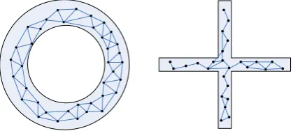
In order to solve this problem, some topology adaptive algorithms have been proposed, such as GNG in Ref. [18], PSOM in Ref. [19], and DASH in Ref. [20]. These algorithms free of predefining neuron topology and can automatically construct it to let it conform to the distribution of input data. We take DASH for example and show the clustering results in Figure 3.
As stated in the introduction, there are two deficiencies of traditional topology adaptive algorithms. One is that they will insert some neurons which locate out of the area where input data distribute. The other is that competitive learning can’t be performed by them. Figure 4 shows the simulation results affected by these two deficiencies.
Although there are some neurons out of the area where input data distribute in Figure 4, it doesn’t hamper us from drawing the conclusion that topology adaptive algorithms can better cluster dynamic data than SOM and its scalable versions. This proof is shown in Figure 5.
Figure 3. Use DASH to form neuron topology to simulate the distribution of the synthetic data in the gray area
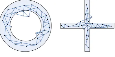
Figure 4. Use DASH to form neuron topology to simulate
the distribution of the synthetic data as round and cross shapes
Figure 5. Use DASH to form neuron topology to simulate
In order to accurately cluster dynamic data which isn’t effectively solved by traditional topology fixed algorithms and topology adaptive algorithms, a novel
Topology Self-Adaptive Clustering algorithm
(abbreviated as TSAC) is proposed in this paper. It can dynamically alter its neuron topology following the update of input data through fulfilling two sub-processes. They are: (a) initialization of neuron topology; (b) training on neuron topology. In the former sub-process, an initial neuron topology is rapidly constructed according to input data, which is partially similar to the distribution of input data. In the latter sub-process, the neuron topology is iteratively altered by training samples to let it gradually conform to the distribution of input data.
3. Topology self-adaptive clustering algorithm (TSAC)
3.1. Initialization of neuron topology
In this section, we will elaborate how to rapidly initialize neuron topology, which is roughly similar to the distribution of input data and only needs a few training steps to make it converge in the next training sub-process.
As indicated by Ref. [21], the general way to expand neuron topology is to combine the neuron which has the largest accumulation error with its least similar neighbor to form a new one. Unfortunately, this plan brings an inconvenient consequence that it may create the neurons which locate out of the area where input data distribute.
For dealing with this issue, TSAC imports local density, proposed by Duan et al. in Ref. [22], to construct the new neuron.
Let Di represent one datum among input data. The
neuron which is constructed from Di is marked as Ni.
The process that constructs Ni from Di by local density
is shown as follows:
Choose t samples from input data, where t is decided by user. Among them, the kth sample has kth similarity to Di. Calculate local density of Di and each
sample among those t data by
1
( )
( ( , ))
( )
m
ik ik r
ik
Density SD Density Neighbor SD r LocalDensity SD
m
, (1)where SDik represents the datum which has kth
similarity to Di. Neighbor(SDik,r) represents the datum
which has rth similarity to SDik. m represents the
quantity of the neighbors which are adjacent to SDik,
and it often equals to t. Density(SDik) represents the
density of the district around SDik, and can be
calculated by
2
1
| ( , ) |
( )
m
ik ik
r ik
SD Neighbor SD r
Density SD
m
. (2)After previous calculations, treat the datum, which has the maximal local density, as the neuron to represent the cluster which includes Di.
The detailed procedure of initialization sub-process of TSAC is listed as follows.
1. Arrange input data by random order, and put them in the set marked as InSet. Let the symbol
NEURON stand for the neuron set. Let the symbol
LINK stand for the set which includes the links between different neurons, where each link has two parameters, which are relation to express its weight and age to note its creating time.
2. Choose two data from Inset which has the minimal similarity, and mark them as Dp and Dq. Apply
previous local density plan to construct two neurons from them, and mark them as Np and Nq.
Insert them in NEURON. Remove Dp and Dq from
Inset.
3. Create a link between Np and Nq, mark it as lpq,
and insert it in LINK. Mark time parameter of lpq
as Agepq, and assign it with 0. Mark relation
parameter of lpq as Rpq, and calculate it by
2 1 1
pq pq
C C pq p q
Sim R
Sim
, (3)
where C represents the quantity of the clusters, which equals to the number of the neurons. Simpq
represents the similarity between two neurons, such as Np and Nq.
2
1
( )
| | *
( )
z p
pq pk qk
q k
LocalDensity N
Sim W W
LocalDensity N
, (4)where z represents the dimension of neuron vector,
Wpk represents the weight of kth entry in Np.
Traditional concurrence based similarity calculations, e.g. Euclidean distance or Cosine, have a flaw that the neurons, which locate at the two opposite boundaries of the same cluster, have less similarity, if the similarity is calculated by them. Actually, those neurons should have larger similarity, because they are in the same cluster. Thus, we integrate local density into Eq.4 to deal with this shortcoming.
4. Scan InSet from top to bottom, mark Di as the
datum which is just selected, and remove it from
InSet. Use previous local density plan to construct one neuronfrom Di, and mark it as Ni. Insert Ni in
NEURON.
5. Apply Eq.4 to calculate the similarity between Ni
and each neuron in NEURON.
6. Let Nm represent the neuron which has the
maximal similarity to Ni in NEURON. Create a
link between Ni and Nm, mark it as lim, and insertit
in LINK. Assign the age parameter-Ageim of lim
with 0. Calculate the relation parameter-Rim of lim
7. If the similarity between Ni and Nm is beyond
certain threshold, such as the mean of the total similarities among all the neuron-pairs, go to step [8]. If not, go to step [12].
8. Tune Nm by
1
exp( )* z | |
m m im ik mk
k
N N R N N
. (5)This equation is just borrowed from Ref. [23]. Where, z represents the number of the neurons, Rim
represents the relation value between two neurons of Ni and Nm, acquired by Eq.3.
9. Choose the neuron from NEURON which has the secondly maximal similarity to Ni,and mark it as
Nj.
10. If there is no link between Nj and Nm, go to step
[11]. If not, go to step [12].
11. Create a link between Nj and Nm, mark it as ljm,
and insertit in LINK.
12. Apply Eq.3 to calculate the relation parameter-Rjm
of link ljm. Assign the age parameter-Agejm of ljm
with 0.
13. Add age parameters of all the links to 1. If there is a link whose age parameter is beyond the threshold calculated by the following equation, remove it.
x
/ ( / )i Tma
u u d
Threshold T T T , (6)
where i represents the index of running steps. Tu,
Td, Tmax are respectively evaluated with 20, 200,
10000. Those values are validated by a large amount of experiments and exhibited in Ref. [23]. Apparently, along with proceeding of initialization sub-process, the threshold of age parameter calculated by Eq.6 becomes larger and larger. The reason is that, along with continuing of initialization sub-process, cluster partition is more and more accurate, thus, the links between different neurons should maintain stable. Therefore, we gradually increase the threshold of age parameter to make the links difficult to be deleted.
14 Choose i+1th datum from InSet, and repeat steps [4] ~ [14] until InSet is empty.
Figure 6 shows the neuron topology formed after initialization sub-process. It is easy to see, the neuron topology is partially similar to the distribution of the synthetic data. For example, certain area has too many neurons, and certain area has few neurons.
3.2. Training on neuron topology
As Figure 6 shows, the neuron topology formed after initialization sub-process is inaccurate. In order
Figure 6. Neuron topology formed by TSAC after
initialization sub-process
to amend it, we add a training process, and import competitive learning proposed by Ref. [24] into it.
Due to lacking of topology order, the adjacent neurons of the winner neuron (the neuron which has the maximal similarity to training sample) can’t be found by traditional topology adaptive algorithms to perform competitive learning. Since our algorithm is also a kind of topology adaptive algorithms, we employ minimum spanning tree addressed by Ref. [25] to form topology order. The minimum spanning tree formed by TSAC after training sub-process is shown in Figure 7. It is easy to see, the structure of minimum spanning tree is similar to the distribution of the synthetic data.
Figure 7. Minimum spanning trees formed by TSAC after
training sub-process, where the dots represent the neurons and the links represent the arcs of the tree
In virtue of minimum spanning tree, we can define neuron adjustment range in the following equation, which is never carried out by traditional topology adaptive algorithms.
2 m
( , ) ( ) * max(| | ) b
b N
m t a t N N
, (7)
where Nm represents the winner neuron. ε represents
the set which includes the neurons that are directly connected to Nm in the minimum spanning tree, such
as Nb. a(t) is learning rate.
By means of neuron adjustment range, we can tune the neurons by
1) () ()*exp( (t N t at NLb b
)]; ( [
* ) ) , (
2 2 mt D N t
R
b i
bm
) , (mt
where Nmrepresents the winner neuron which has the
maximal similarity to Di. Rbmis the relation value
between Nmand Nb, which can be acquired by Eq.3. t
represents the index of training steps. a(t) is learning rate which monotonously drops along with training process, and is specified in Ref. [26].
So, why we choose the neurons, which are directly connected to the winner neuron, to form neuron’s adjustment range? The reason is proved as follows.
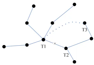
Theorem: The neurons which are directly connected
to the winner neuron are more similar to the winner neuron than to other neurons. ▼Proof: Let Tree1 represent the minimum
spanning tree displayed in Figure 8, where each node represents one neuron. Let T1 represent the winner neuron, and T2 represent the neuron which is directly connected to T1. Let ARCT1T2 represent the arc linking
T1 and T2. Let RT1T2 represent the relation parameter
of ARCT1T2 acquired by Eq.3. Let WAT1T2 represent the
weight of ARCT1T2. Since we reverse the value of the
relation parameter as the weight of the arc, WAT1T2=1/
RT1T2.
In order to prove this theorem is valid, we can prove its opposite assumption is false. If we assume this theorem were invalid, we can find a neuron, labeled by T3, which is directly connected to T2 but not directly connected to T1. After connect T1 to T3 by the dotted line in Tree1, we will have
1 2 1 3
T T T T
R R orWAT T1 2WAT T1 3. It means T3 is
more similar to T1 than to T2.
Apparently, after connect T1 to T3, there will be a circle through T1, T2 and T3 in Tree1. If we remove the arc linking T1 and T2, there will be a new tree and we label it as Tree2. According to the assumption that
1 2 1 3
T T T T
WA WA , the weight of Tree1 is bigger than that of Tree2. However, Tree1 is the minimum spanning tree through T1, T2 and T3. Thus, the assumption thatRT T1 2RT T1 3 or WAT T1 2WAT T1 3
is false. Then, we can say that the aforementioned theorem we are just proving is valid. ▲
Figure 8. Minimum spanning tree of neuron topology
The detailed procedure of training sub-process of TSAC is listed as follows.
1. Mark the neuron set and the link set formed from initialization sub-process as NEURON and LINK. Initialize error coefficient of each neuron with 0. Let Inset represent the set containing input data.
Let t represent the index of training steps, and initialize itwith 0.
2. Randomly choose a datum from Inset, and mark it as Di. Calculate the similarity between Di and each
neuron in NEURON by Eq.4.
3. Choose the neuron which has the maximal similarity to Di as the winter neuron, and mark it
as MBN. Tune MBN and its adjacent neurons by Eq.8. Increase the error coefficient of MBN by
2
| |
m m i
err err DMBN , (9)
where, errm represents the error coefficient of
MBN.
4. Choose the neuron which has the secondly maximal similarity to Di, and mark it as SBN. If
there is no link between MBN and SBN, go to [5]. If not, go to [6].
5. Create a link between MBN and SBN, mark it as
lms, and insert it in LINK.
6. Apply Eq.3 to calculate the relation parameter-Rms
of lms. Assign age parameter-Agems of lms with 0.
7. Add age parameters of all the links in LINK to 1. 8. Check each link in LINK. If there is a link whose
age parameter is beyond the threshold calculated by Eq.6, remove it.
9. Check each neuron in NEURON. If there is a neuron which isn’t connected by any link, remove it.
10. Increase t to t+1.
11. If t is the integral times of the quantity of input data, go to step [12]. If not, go to step [2].
12. Choose the neuron which has the maximal error coefficient, and mark it as Nq. Choose the neuron
which is adjacent to Nq and has the minimal
similarity to Nq, and mark it as Nf.
13. Combine Nq and Nf to construct a new neuron by
2
q f
r N N
N (10)
Mark this created neuron as Nr. Create the links
between Nq andNr, Nfand Nr, and insert them in
LINK. Initialize age parameter of each newly created link with 0.
14. Reduce error coefficients of Nq andNf by / 2
q q
err err , (11)
/ 2
f f
err err . (12)
Assign Nr with the new error coefficient by
2
q f r err err
err . (13)
Neuron topology formed after training sub-process is shown in Figure 9. Comparing Figure 6 with Figure 9, it can be concluded that, by dynamically creating and removing the neurons, the neuron topology displayed in Figure 9 is more identical with the distribution of the synthetic data than that displayed in Figure 6.
Figure 9. Neuron topology formed by TSAC after training
sub-process
Since only the winner neuron and its adjacent neurons of small number are adjusted in each circulation of training sub-process, it makes the entire neuron topology change very slightly after each training circulation. Thus, there is no need to construct minimum spanning tree again after each training circulation. For this reason, when TSAC runs for about the integral times of 100 training circulations, minimum spanning tree is constructed once more.
In our algorithm, Mean Quantization Error
(abbreviated as MQE) is adopted as convergence condition as performed by many literatures [15~17]. Since MQE can measure the average agglomeration degree of clustering results, when its value is less than a threshold such as 0.01 (which is adopted by Kohonen in Ref. [27]), our algorithm stops.
2
1
|
-
|
|
|
i j
C
i j
j j D C
D N
C
MQE
C
, (14)where C represents the quantity of the clusters. Nj
represents one neuron. Cj represents the cluster,
including the texts which are more similar to Nj than
to other neurons. |Cj| represents the quantity of the
data included by Cj. Direpresents one datum among
Cj.
4. Data evolvement analysis
In this paper, TSAC is applied to perform data evolvement analysis to help users apprehend the transfer of the information expressed by the data sets collected in different time phases, which also demonstrates that TSAC can cluster dynamic data on the other side.
4.1. The process to cluster dynamic data
For helping explain how to cluster dynamic data, let’s adopt some symbols. Let t1 and t2 represent two
time phases. Let InSett1 and InSett1 represent the data
sets respectively collected in t1 and t2. For clustering
the dynamic data from t1 to t2,we first use TSAC to
form a neuron topology according to InSett1. When
InSett1 is updated, for example, changing to InSett2,
we use TSAC to alter the existent neuron topology according to InSett2. The altering process is just the
same to the training sub-process of TSAC. Once data set is updated again, it only needs to run this training sub-process once more to alter the existent neuron topology according to the updated data set.
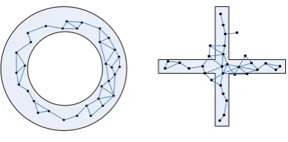
From Figure 10, it is easy to find, when input data are updated, neuron topology is reconstructed to simulate the distribution of the updated data.
Figure 10. Use TSAC to form neuron topology to simulate
the distribution of the synthetic data. For simulating dynamic data, we partition the circle into three rings marked
as R1, R2, and R3 form inside to outside. We firstly use the data in R1 and R2 to form a neuron topology by TSAC, and the result is shown in the left picture. After that, we use the
data in R2 and R3 to alter this neuron topology, and the result is shown in the right picture
4.2. Grid analysis
Grid structure is applied to measure the transfer of the information expressed by the data sets collected in different time phases.
At first, data space is partitioned into some grids. The scale of each dimension of each grid is
. After partition, the neurons are projected into those grids. As indicated by Herbert and Yao in Ref. [28], each neuron represents one cluster which aggregates similar data, and the data included by the clusters represented by the adjacent neurons are also similar to each other. Hence, the clusters represented by the neurons in the same grid should imply similar information. Consequently, the quantity of the neurons contained by each grid can be used to measure the importance of the information expressed by the data included by this grid.Obviously,λcontrols the range of each grid. Ifλ is larger, each grid will include more neurons and we can make analysis more comprehensively. On the other side, if λ is smaller, we can make analysis more particularly.
Let Gt1 represent the grid structure constructed in
t1. Let Gt2 represent the grid structure constructed in t2.
We can acquire the knowledge about the transfer of the information from t1 to t2 through digging the
measuring the transfer, we calculate the density of each grid in Gt1by
1
1 1
| |
2 1
( ( )) ( ( ))
( ( ))
i i
Gt
i i
Number P Gt Denstiy P Gt
Number P Gt
, (15)
where Pi(Gt1) represents one grid in Gt1.
Number(Pi(Gt1)) represents the quantity of the neurons
included by Pi(Gt1). |Gt1| represents the quantity of the
grids included by Gt1. The density of each grid in Gt2
can also be calculated by this equation.
For measuring the transfer of the information, we set a threshold in advance, and consider the information expressed by the data in the grid which is beyond the threshold is more important. The density threshold is set as the mean density through all the grids. Let DGt1 and DGt2 respectively represent the
sets storing the dense grids in Gt1and Gt2. Then, we
can acquire the following three subsets: DGt1DGt2 , DGt2DGt1 , DGt1DGt2 .
Among them, DGt1DGt2 implies the information,
which appears at t1 and disappears at t2; DGt2DGt1
implies the information, which newly appears at t2;
1 2
DGt DGt implies the information, which keeps from t1 to t2.
5. Experiments and analysis
5.1. Experiments on clustering performance
As indicated by Ref. [29], UCI data set is one of the most prevalent testing corpora for clustering algorithms. Since it contains too many kinds of data sets, we only select some extensively applied sets as the standard testing corpus to compare the performance of TSAC with that of other clustering algorithms. They are GNG [18], PSOM [19], DASH [20], SOM [15], GSOM [16], and GHSOM [17]. The details about the selected sets are listed in Table 1.
Table 1. The details about the selected data sets from UCI data set
#DATA SETS #Features #Samples #Classes
Thyroid Gland 5 215 3
Japanese Credit Approval 15 688 2
Wine Recognition 13 178 3
Breast Cancer 10 699 2
Iris 4 150 3
Sonar Target 60 208 2
Ionosphere 34 51 2
Heart Disease 13 135 2
Waveform 21 5000 3
Pima Diabetes 8 768 2
Multiple Feature 649 2000 10
Optical Digit 64 5620 10
German Credit Approval 24 1000 2
Car Evaluation 6 1728 4
Purity, indicated by Ref. [30], is employed as the testing criterion, and calculated by
1
( ) z
r r r
n
Purity P S
n
, (16)where z represents the quantity of the clusters. n
represents the quantity of input data. Sr represents rth
cluster formed by clustering algorithm. nr represents
the quantity of the data included by Sr. P(Sr) is
calculated by
1 1
( ) max( )z q
r q r
r
P S n
n
. (17)
In UCI, it already partitions the testing data into some predefined clusters. Thus, let Cq represent qth cluster
among the predefined clusters. Let nq represent the
quantity of the data included by Cq.
n n
rq=
q
n
r ,which represents the quantity of the data, belonging to
Cq in testing corpus and belonging to Sr after
clustering algorithm.
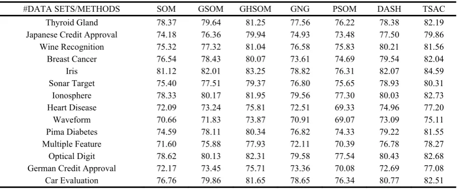
Table 2. Purities of different clustering algorithms on the selected data sets
#DATA SETS/METHODS SOM GSOM GHSOM GNG PSOM DASH TSAC
Thyroid Gland 78.37 79.64 81.25 77.56 76.22 78.38 82.19
Japanese Credit Approval 74.18 76.36 79.94 74.93 73.48 77.50 79.86
Wine Recognition 75.32 77.32 81.04 76.58 75.83 80.21 81.56
Breast Cancer 76.54 78.43 80.07 73.61 74.69 79.54 82.04
Iris 81.12 82.01 83.25 78.82 76.31 82.07 84.59
Sonar Target 75.40 77.51 79.37 76.80 75.65 78.93 80.31
Ionosphere 78.33 80.17 81.95 79.56 77.30 80.03 82.73
Heart Disease 72.09 73.24 75.81 72.51 69.33 74.96 77.20
Waveform 70.66 71.83 73.87 70.91 69.07 73.09 75.11
Pima Diabetes 74.59 78.11 80.34 76.82 74.33 79.22 81.55
Multiple Feature 71.60 75.88 77.93 72.11 70.39 76.78 78.27
Optical Digit 78.62 80.13 82.31 79.58 77.54 80.43 82.68
German Credit Approval 72.17 73.45 75.71 73.36 70.08 72.69 77.08
Obviously, TSAC has the best performance than any other clustering algorithm. This is because, it doesn’t need to perform any assumption about neuron topology beforehand, and can dynamically form it according to input data. Besides, to further boost its performance, it constructs minimum spanning tree to perform competitive learning. Through pervious operations, TSAC can simulate the distribution of input data very well, and consequently has the best performance.
5.2. Experiments on data evolvement analysis
The data from UCI set don’t change along with time passing. Therefore, we can’t utilize them to test the performance of TSAC for dynamic data. For this reason, we crawl ten thousands news webpages from website over the entire year of 2010 as testing corpus, and separate it into two sets to represent the dynamic data collected in two time phases. Let InSett1 represent
the set which includes the news from January to June. Let InSett2 represent the set which includes the news
from July to December.
As indicated in the section 4.1, data evolvement analysis performed by TSAC has two steps. In the former step, it clusters InSett1 to form neuron
topology. In the latter step, it alters neuron topology according to InSett2. For measuring the transfer of the
information expressed by the data in InSett1 and
InSett2, we partition the neuron topologies respectively
formed by InSett1 and InSett2 into some grids, and
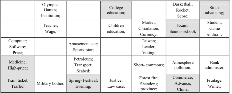
extract the labels to represent the information expressed by the data in each grid. The grid structure and its labels are shown in Table 3.
In Table 3, the grid colored with gray means the information expressed by the data in this grid is important. The grid colored with white means the information expressed by the data in this grid is little important. The blank grid means the information expressed by the data in this grid isn’t important in table (a) but appears or becomes important in sub-table (b), or on the contrary.
Table 3 (a). The grids constructed from the news sampled from January to June
Microsoft; Operation;
Football; Club title;
College education;
Missile; Defense;
Basketball; Rocket;
Score;
Stock advancing;
America; Afghanistan;
Conflict;
Payment; Innovation;
Improve;
Market; Circulation;
Currency; Phone;
Apple; Quality;
Amusement star; Sports star;
Africa; Diamond;
U.N.; Seat;
Fashion; Dress;
Medicine; High-price;
Car; Sell;
Diving;
Champion; Short- commons;
Spring- Festival; Evening;
Commerce; Advance;
China;
Table 3 (b). The grids constructed from the news sampled from July to December
Olympic- Games; Institution;
College education;
Basketball; Rocket;
Score;
Stock advancing;
Teacher; Wage;
Children education;
Market; Circulation;
Currency;
Exam; Senior- school;
Student; Game enthrall; Computer;
Software; Price;
Amusement star; Sports star;
Taiwan; Leader; Voting; Medicine;
High-price;
Petroleum; Transport; Seabed;
Short- commons; Atmosphere pollution; administer; Bank
Train ticket;
Traffic; Military bother;
Spring- Festival; Evening;
Justice; Law case;
Forest fire; Shandong
province;
Commerce; Advance;
China;
In comparison with two sub-tables of Table 3, we can see that some information which sub-table (a) labels has disappeared in sub-table (b) such as
confliction between America and Afghanistan. Some information which sub-table (a) doesn’t label has appeared in sub-table (b), such as leader voting in Taiwan. Some information which labels in sub-table (a) has changed their importance in sub-table (b), such as advance of stock. There is also some information which keeps its importance form table (a) to sub-table (b), such as score of Rocket team in basketball. Previous results explicitly illustrate that TSAC can detect the transfer of the information when input data are updated.
6. Conclusions
Along with the fast advance of internet technique, new information appears every day. In order to apprehend the transfer of the information expressed by the data collected in different time phases, a novel topology adaptive clustering algorithm is proposed in this paper, which is abbreviated as TSAC. This algorithm doesn’t need to make any assumption about neuron topology in advance, and can dynamically form it to simulate the distribution of input data. For avoiding the neurons from locating out of the area where input data distribute, it adopts local density to construct new neurons. Besides, minimum spanning tree is imported to perform competitive learning to further enhance its performance. Experiment results demonstrate that TSAC works better than most of traditional clustering algorithms. Another ability of TSAC is that it can cluster dynamic data. For illustrating it, TSAC is used to display the transfer of the information expressed by the news crawled from website through the entire year of 2011. For quantitatively measuring the transfer, data space is partitioned into several grids and density is adopted as the measure criterion.
Acknowledgements
The research in this paper is supported by National Natural Science Foundation of China (NO. 60973076, 61073127), and Key Laboratory Opening Funding of China MOE-MS Key Laboratory of Natural Language Processing and Speech.
References
[1] S. Martin, N. Detlef. Towards the automation of
intelligent data analysis. In: Applied Soft Computing, vol. 6, no. 4, pp. 348-356, 2006. http://dx.doi.org/ 10.1016/j.asoc.2005.11.002.
[2] X.-Y. Zhou, Z.-H. Sun, B.-L. Zhang, Y.-D. Yang.
Research on clustering and evolution analysis of high dimensional data stream. In: Journal of Computer Research and Development, vol. 43, pp. 2005-2011, 2006. http://dx.doi.org/10.1360/crad20061122.
[3] I.-D. Alfonso, P. Francesco, G. Michael. Exploratory data analysis leading towards the most interesting simple association rules. In: Computational Statistics & Data Analysis, vol. 52, no. 6, pp. 3269-3281, 2008. http://dx.doi.org/10.1016/j.csda.2007.10.006.
[4] H.-G. Silber, K.-F. McCoy. Efficiently computed
lexical chains as an intermediate representation for automatic text summarization. In: Computational Linguistics, vol. 28, no. 4, pp. 487-496, 2002. http://dx.doi.org/10.1162/089120102762671954.
[5] A. Roberto. Multivariate classification of constrained data: problems and alternatives. In: Analytica Chimica Acta, vol. 527, no. 1, pp. 45-51, 2004. http://dx. doi.org/10.1016/j.aca.2004.07.068.
[6] R. Krishnapuram, A. Joshi, O. Nasraoui, L. Y. Yi.
Low-complexity fuzzy relational clustering algorithms for web mining. In: IEEE Transactions on Fuzzy Systems, vol. 9, no. 4, pp. 595-607, 2001. http://dx. doi.org/10.1109/91.940971.
[7] S. Huang, Z. Chen, Y. Yu, W.-Y. Ma. Multitype
features coselection for web document clustering. In: IEEE Transactions on Knowledge and Data Engineering, vol. 18, no. 4, pp. 448-459, 2006. http://dx.doi.org/10.1109/TKDE.2006.1599384.
[8] D. A. Viattchenin. Validity measures for heuristic
possibilistic clustering. In: Information Technology and Control, Vol. 39, No. 4, pp.321-332, 2010.
[9] I.-S. Dhillon, Y.-Q. Guan, J. Kogan. Iterative
clustering of high dimensional text data augmented by local search. In: Proceedings of the Second IEEE International Conference on Data Mining, IEEE, Maebashi, Japan, pp. 131-138, 2002.
[10] M.-H. Ghaseminezhad, A. Karami. A novel
self-organizing map (SOM) neural network for discrete groups of data clustering. In: Applied Soft Computing, vol. 11, no. 4, pp. 3771-3778, 2011. http://dx.doi.org/ 10.1016/j.asoc.2011.02.009.
[11] Y.-K. Melody. Extending the Kohonen self-organizing map networks for clustering analysis. In: Computational Statistics & Data Analysis, vol. 38, no. 2, pp. 161-180, 2001. http://dx.doi.org/10.1016/S0167-9473(01)00040-8.
[12] C.-L. Tseng, Y.-H. Chen, Y.-Y. Xu, H.-T. Pao, H.-C. Fu. A self-growing probabilistic decision-based neural network with automatic data clustering. In: Neurocomputing, vol. 61, pp. 21-38, 2004. http:// dx.doi.org/10.1016/j.neucom.2004.03.002.
[13] C.-F. Tsai, C.-W. Tsai, H.-C. Wu, T. Yang. ACODF: a novel data clustering approach for data mining in large databases. In: Journal of Systems and Software, vol. 73, no. 1, pp. 133-145, 2004. http://dx.doi.org/10. 1016/S0164-1212(03)00216-4.
[14] S. Lee, G. Kim, S. Kim. Self-adaptive and dynamic
clustering for online anomaly detection. In: Expert Systems with Applications, vol. 38, no. 12, pp. 14891-14898, 2011. http://dx.doi.org/10.1016/j.eswa.2011 .05.058.
[15] T. Kohonen. “Self-organizing maps”. Springer,
Berlin, 1995, (Second, Extended Edition 1997).
[16] D. Alahakoon, S.-K. Halganmuge, B. Srinivasan.
[17] A. Rauber, D. Merkl, M. Dittenbach. The growing hierarchical self-organizing map: exploratory analysis of high-dimensional data. In: IEEE Transactions on Neural Networks, vol. 13, no. 6, pp. 1331-1341, 2002. http://dx.doi.org/10.1109/TNN.2002.804221.
[18] A.-K. Qin, P.-N. Suganthan. Robust growing neural
gas algorithm with application in cluster analysis. In: Neural Networks, vol. 17, no. 8-9, pp. 1135-1148, 2004.
[19] L.-K. Robert, K. Warwick. The plastic self
organising map. In: Proceedings of the 2002 International Joint Conference on Neural Networks, IEEE, Hawaii, pp. 727-732, 2002.
[20] C. Hung, S. Wermter. A dynamic adaptive
self-organising hybrid model for text clustering. In: Proceedings of the Third IEEE International Conference on Data Mining, IEEE, Melbourne, Florida, USA, pp. 75-82, 2003. http://dx.doi.org/ 10.1109/ICDM.2003.1250905.
[21] V.-J. Hodge, J. Austin. Hierarchical growing cell
structures: TreeGCS. In: IEEE Transactions on Knowledge and Data Engineering, vol. 13, no. 2, pp. 207-218, 2001. http://dx.doi.org/10.1109/69.917561.
[22] L. Duan, L.-D. Xu, F. Guo, J. Lee, B.-P. Yan. A
local-density based spatial clustering algorithm with noise. In: Information Systems, vol. 32, no. 7, pp. 978-986, 2007. http://dx.doi.org/10.1016/j.is.2006.10.006.
[23] H. Barbara, M. Alessio, S. Alessandro, S. Marc.
Recursive self-organizing network models. In: Neural Networks, vol. 17, no. 8-9, pp. 1061-1085, 2004. http://dx.doi.org/10.1016/j.neunet.2004.06.009.
[24] H.-D. Jin, W.-H. Shum, K.-S. Leung, M.-L. Wong.
Expanding self-organizing map for data visualization and cluster analysis. In: Information Sciences, vol. 163, no. 1-3, pp. 157-173, 2004. http://dx.doi.org/ 10.1016/j.ins.2003.03.020.
[25] L.-R. Ezequiel. Probabilistic self-organizing maps for qualitative data. In: Neural Networks, vol. 23, no. 10, pp. 1208-1225, 2010. http://dx.doi.org/10.1016/ j.neunet.2010.07.002.
[26] K. Tokunaga, T. Furukawa. Modular network SOM. In: Neural Networks, vol. 22, no. 1, pp. 82-90, 2009. http://dx.doi.org/10.1016/j.neunet.2008.10.006.
[27] T. Kohonen, S. Kaski, K. Lagus, J. Salojarvi, V. Paatero, A. Saarela. Self organization of a massive
document collection. In: IEEE Transactions on Neural Networks, vol. 11, no. 3, pp. 574-585, 2000. http://dx.doi.org/10.1109/72.846729.
[28] J.-P. Herbert, J.-T. Yao. A granular computing
framework for self-organizing maps. In: Neurocomputing, vol. 72, no. 13-15, pp. 2865-2872, 2009. http://dx.doi.org/10.1016/j.neucom.2008.06.031.
[29] C. Blake, E. Keogh, C.-J. Merz. UCI repository of
machine learning databases. In: http://www.ics.uci.edu /~mlearn/MLRepository.html, Irvine, CA: University of California, 1998.
[30] M. Gu, H. Zha, C. Ding, X. He, H. Simon, J. Xia.