The Application of the Root Locus Method for the Design of Pitch Controller of an F-104A Aircraft

The Application of the Root Locus Method for the Design of

Pitch Controller of an F-104A Aircraft

Branimir Stojiljković1 _{- Ljubiša Vasov}1 _{- Časlav Mitrović}2 _{- Dragan Cvetković}3,* 1 _{University of Belgrade, Faculty of Transport and Traffic Engineering, Serbia}

2 _{University of Belgrade, Faculty of Mechanical Engineering, Serbia}

3 _{University ''Singidunum'' Belgrade, Faculty of Informatics and Management, Serbia}

This paper presents an application of the root locus technique for the design of a feedback control system of an F-104A aircraft. The analysis of the longitudinal aircraft stability was performed for the Single Input Single Output (SISO) open-loop system, using linearised equations of aircraft motion and aerodynamic derivatives of an F-104A aircraft taken from the NASA report [1]. The dynamical behavior of the open-loop system was unsatisfactory and led to the introduction of the feedback control system. The closed-loop system was designed using the root locus technique, developed by Evans in 1948. The transfer function parameters of each element of the feedback control system are determined according to previously set design requirements. Although, the analysis of the closed-loop step response showed that all of the design requirements were realised, the controller designed within the proposed control system structure is not the only one, and there are different controller designs that lead to a satisfactory solution.

© 2009 Journal of Mechanical Engineering. All rights reserved.

Keywords: controller synthesis, root locus, stability derivatives, longitudinal dynamical stability

0 INTRODUCTION

Modern aircraft include automatic control systems that aid the flight crew in navigation, flight management and provide artificial stability. Designing an autopilot requires control systems theory background and knowledge of stability derivatives at different altitudes and Mach numbers for a given airplane. The stability derivatives can be obtained from wind tunnel or in-flight tests, and are usualy given for a body-fixed axis system aligned with the fuselage reference line or stability axis system aligned with the projection of the total steady-state velocity vector on the aircraft’s plane of symmetry.

Each component of the control system is defined in terms of its transfer function. The transfer functions relating the aircraft’s response to control inputs are determined from the equations of aircraft motion and represent functions of dimensional stability derivatives, geometric, mass and flight condition parameters. The simplest form of the control system is an open-loop system in which the control action is independent of the output. In order to obtain a more accurate control system, the connection between the output and input signal must be established, forming a closed-loop feedback

control system composed of a comparator, a controller and a control object. The controller design process called controller synthesis must assure dynamical stability and wanted dynamical behavior of a system expressed through response characteristics of a system.

The root locus technique is one of the design analysis tools used in this paper for controller synthesis of an F-104A aircraft. The dimensional stability derivatives are taken from the NASA report no. CR-2144 named “Aircraft handling qualities data“ [1], to obtain the longitudinal transfer function neccesary for dynamical stability analysis.

1 EQUATIONS OF LONGITUDINAL AIRCRAFT MOTION

The first step in control system analysis is defining a mathematical model which contains all the essential information about the physical properties of a given system, so that research of a physical system can be carried out on its mathematical model. The mathematical model of a physical system is described by differential equations, which are usually given in the following state-space form:

,

y Cx Du= + ₍₂₎ where x, u and y are state, input and output vectors, and A, B, C and D are state, input, output and feedthrough matrices.

The equations of aircraft motion are obtained from Newton’s second law, which is referred to an absolute or inertial reference frame. In general, aircraft motion can be viewed as a combination of translatory motion of airplane’s center of mass, governed by the force equation, and rotary aircraft motion about its center of mass, governed by the moment equation. The orientation of the airplane is described using Euler’s angles. For many problems in airplane dynamics, an axis system fixed to the Earth can be used as an inertial reference frame. Unfortunately, the moments and products of inertia included in the moment equation will vary with time as the airplane rotates. To avoid this problem the equations of airplane motion are usually derived for an axis system fixed to an airplane called body axis system. These equations are nonlinear but can be linearised using small-disturbance theory, which assumes that the motion of an airplane consists of small deviations about a steady flight condition. Depending on the assumed flight condition the complete set of linearised equations of aircraft motion can be separated into two independent sets: longitudinal and lateral set of equations. The equations of longitudinal aircraft motion are obtained assuming symmetric reference flight condition.

This paper analyses dynamical behaviour of an aircraft in symmetric reference flight

condition, regarding time change of pitch angle as output variable caused by a step change of control surface deflection angle, as input variable. If the state vector for an aircraft in this SISO open-loop system is defined as:

, u w x q θ ⎛ ⎞ ⎜ ⎟ ⎜ ⎟ =_{⎜ ⎟} ⎜ ⎟ ⎝ ⎠ (3)

where the state variables u, w, q and θ represent the perturbations from an equilibrium condition of forward velocity, yaw velocity, pitch rate, and pitch angle, and if the aircraft is being controlled by means of stabilizer deflection δs, then the state-space form of longitudinal equations of aircraft motion is defined as:

( )

u u

w w

A B

q q δ

θ θ ⎛ ⎞ ⎛ ⎞ ⎜ ⎟ ⎜ ⎟ ⎜ ⎟₌ ⎜ ⎟₊ ⎜ ⎟ ⎜ ⎟ ⎜ ⎟ ⎜ ⎟ ⎝ ⎠ ⎝ ⎠ & & & & (4)

( )

( )

u w C D q θ δ θ ⎛ ⎞ ⎜ ⎟ ⎜ ⎟ = + ⎜ ⎟ ⎜ ⎟ ⎝ ⎠ (5)

Matrices A and B are functions of steady-state flight parameter values (u0, w0, θ0) and

stability derivatives of an aircraft, which are evaluated at the reference flight condition:

* _cos

0 0

* _sin

0 ₀

1 1 1 1

* _{( ) sin}

0

* 0

( ) ( ) ( ) ( )

1 1 1 1

0 0 1 0

X_u X_w w g

Z u

Z Z _q g

u w

Z Z Z Z

w w w w

A

Z u M

Z M_{u w} Z M_{w w q w} g

M M M M

u Z w Z q Z Z w

w w w w

θ θ θ ⎛ _{− −} ⎞ ⎜ ⎟ ⎜ ₊ ⎟ − ⎜ ⎟ ⎜ ⎟ − − − − ⎜ ⎟ = ⎜ ⎟ + ⎜ − ⎟ ⎜ _{+ + +} ⎟ ⎜ − − − − ⎟ ⎜ ⎟ ⎜ ⎟ ⎝ ⎠

& & & &

& & &

&

& & & &

Considering SISO open-loop system matrices C and D are defined as:

(

)

C= (8)

( )

D= ₍₉₎

Substituting values of dimensional longitudinal stability derivatives obtained from NASA report no. CR-2144 into state and input matrices, the following linear differential equations are defined:

-0.0117 0.0556 -31.1601 -32.1544 -0.0332 -1.65 892.3082 -1.1229

0.0008 -0.0295 -1.7675 0.0007

0 0 1 0

8.07 -231

-37.766 0 u

w q

u w q

θ

θ

⎛ ⎞ ⎜ ⎟ ⎜ ⎟ = ⎜ ⎟ ⎜ ⎟ ⎝ ⎠

⎛ ⎞⎛ ⎞

⎜ ⎟⎜ ⎟

⎜ _{⎟⎜ ⎟+}

⎜ ⎟⎜ ⎟

⎜ ⎟⎜ ⎟

⎝ ⎠⎝ ⎠

& & & &

( )

⎛ ⎞

⎜ ⎟

⎜ ⎟

⎜ ⎟

⎜ ⎟

⎝ ⎠ (10)

which model the longitudinal motions of the F-104A aircraft about the following equilibrium flight conditions:

Altitude: 0 m (sea level)

Speed: 0.8 Mach = 529 knots = 892.8 m/s Trimmed pitch angle: 2 deg.

2 DYNAMICAL STABILITY ANALYSIS

Dynamical stability analysis is performed in the following section using Matlab software for examining the roots of the characteristic equation. The function ss is used for creating state-space

model within the Matlab enviroment, which takes the model data as input and produces ss object

that store this data in a single Matlab variable. A representation of longitudinal aircraft dynamics can be performed by creating new m-file with the following commands:

A=[-0.0117 0.0556 -31.1601 -32.1544; -0.0332 -1.6500 892.3082 -1.1229; 0.0008 -0.0295 -1.7675 0.0007; 0 0 1 0]; B=[8.0700; -231.0000; -37.7660; 0]; C=[0 0 0 1];

D=[0];

system=ss(A,B,C,D).

Transfer function WO is obtained using tf function in the following manner:

Wo=tf(system)

Transfer function:

-37.77 s^2-55.93 s-0.7108

--- s^4+3.429s^3+29.31s^2+0.3688s+0.07358.

The following commands calculate the zeros and the poles of transfer function:

zeros=zero(Wo) poles=pole(Wo) zeros = -1.4683 -0.0128 poles =

-1.7084 + 5.1325i -1.7084 - 5.1325i -0.0062 + 0.0498i -0.0062 - 0.0498i.

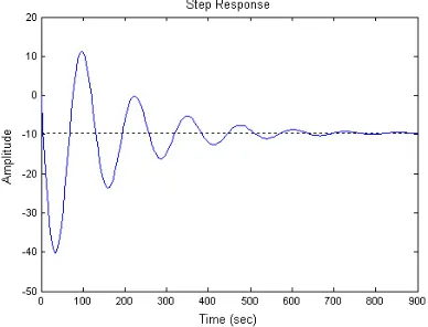
Since all the roots of the characteristic equation have negative real parts, then the system is dynamically stable, and the next step in longitudinal motion analysis is examining the step response. The step response is obtained by typing

step(system) command in the command

window, and presented in Figure 1.

Fig. 1. F-104A open-loop step response

3 CONTROLLER SYNTHESIS

Controller synthesis makes sense only if the system is completely controllable, which means that there exists a control input that transfers any initial state of the system to any final state in some finite time. The test for controllability is applied by calling “controllability.m” file from the command window, which contains the following lines:

A=[-0.0117 0.0556 -31.1601 -32.1544; -0.0332 -1.6500 892.3082 -1.1229; 0.0008 -0.0295 -1.7675 0.0007; 0 0 1 0]; B=[8.0700; -231.0000; -37.7660; 0]; U = ctrb(A, B)

n = length(A) rang = rank(U)

if rang == n

display ('Object is controllable');

else

display ('Object is not

controllable'); end.

The result presented by Matlab looks like this:

U =

1.0e+005 *

0.0001 0.0116 -0.0294 -0.2223 -0.0023 -0.3332 1.2063 5.6279 -0.0004 0.0007 0.0085 -0.0507 0 -0.0004 0.0007 0.0085

n = 4

rang = 4

Object is controllable.

Before continuing with controller synthesis, it is necessary to set the design requirements which should be accomplished:

• Overshoot: < 10%

• Rise time: < 2 s

• Settling time: < 10 s

• Steady-state error: < 2% .

Controller synthesis can be done using different frequency or time-domain methods. The root locus technique is applied in this paper, the discussion of which is presented below. This

technique provides graphical information in the complex plane on the trajectory of the roots of the characteristic equation for variations in one or more system parameters. Since the roots placement in the complex plane governs the type of the response that can be expected to occur, the ability to view the movement of the roots in the complex plane, as one or more system parameters are varied, turns out to be very useful.

Consider the simple feedback system presented in Figure 2:

Fig. 2. Simple closed-loop control system

The closed-loop transfer function of a feedback control system can be expressed as:

( ) ( )

1 ( ) ( )

O C

O C

W s W s W s W s

+ . (11)

The characteristic equation of the closed-loop system is obtained by setting the denominator of the transfer function equal to zero:

1+W s W s_O( ) _C( ) 0= . (12) The loop transfer function WO(s)WC(s) is a function of a complex variable s, and can be written in the factored form, turning the Eq. (12) into form:

1 2

1 2

( - )( - ) ( - )

1 0

( - )( - ) ( - )

m n

s z s z s z k

s p s p s p …

+ =

… , (13)

where z’s and p’s are the zeros and the poles of the transfer function WO(s), n > m and k is an unknown system parameter. In Eq. (13) pure proportional controller is implied, although the control system can be more complicated. The root locus is the locus of all roots of the closed-loop transfer function as the parameter k is varied. When k = 0, the points on the root locus plot are the poles of the loop transfer function, but when k

= ∞, the points on the root locus are the zeros of the loop transfer function. This means that the roots of the closed-loop transfer function migrate from the poles to the zeros of the loop transfer function as k is varied from 0 to ∞. The closed-loop transfer function must have n poles, where n

branches, where each branch starts at a pole and ends at a zero of the loop transfer function. The number of branches of the root locus that go to infinity is equal to the number of zeros at infinity which is determined by the difference between the number of poles and zeros n-m.

The roots of the closed-loop characteristic equation are obtained using graphical-user interface (GUI) within Matlab named SISO Design Tool, designated for controller design using root locus technique, among others. At the beginning, a designer can pick one of the feedback control system structures, and import transfer functions from Matlab’s workspace. In this paper the following feedback structure is used:

Fig. 3. Closed-loop F-104A controller structure

The root locus plot for pure proportional controller (WC(s) = 1, WF(s) = 1) is presented in Figure 4.

Fig. 4. Root locus plot for proportional controller

Design requirements are implemented in the root locus plot in the form of design constraints, represented by one vertical and two lines in an angle. The vertical line indicates the locations of constant settling time and divides the complex plane into the left region, where the

settling time is less than 2s, and the right region, where the settling time is greater than specified. Two lines in an angle indicate the locations of constant overshoot, and the overshoot is less than 10% in between these lines. From examining Figure 4, it can be noticed that the right branches of the root locus are outside the desired region, while the left branches are mainly inside the desired region. Since the displacement of the closed-loop poles along the left branches affect the position of the poles along the right branches, it is impossible to bring all the poles inside the desired region, and, therefore, the root locus must be shifted more to the left by modifying the controller transfer function. This can be done using lead compensator represented by the following transfer function:

0 0

( )

( )

( )

C C

s z W s k

s p − =

− , (14)

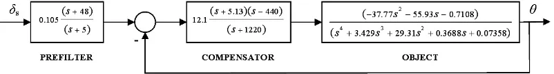
where z0, p0, kC, are zero, pole and gain of the compensator transfer function, and z0 < p0. The first step in controller synthesis was introducing the lead compensator by choosing the numerical values z0 = -5 for the zero, and p0 = -1220 for the pole of the compensator transfer function, and examining the root locus and the closed-loop step response plots. The system was dynamically stable, but the design requirements were not accomplished yet. The second step was adding another real zero to the compensator transfer function z1 = 440, and tunning the compensator gain value around kC = 12, which provided reasonable step response that needed few adjustments carried out by introducing the lag compensator into the prefilter transfer function as a third step of this controller synthesis. The values chosen for the zero and the pole of the prefilter transfer function were zF = -48 and pF = -5. The final step was to pick the value for the prefilter gain kF = 0.105 and execute the final adjustments of the compensator gain kC = 12.1, and the first zero position z0 = -5.13, which led to the following closed-loop system structure:

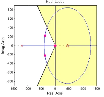
The root locus and the closed-loop step response plot of the feedback system defined in Fig. 5 are presented in the Figs 6. and 7.

Fig. 6. Root locus plot for closed-loop F-104A controller

Fig. 7. F-104A Closed-loop step response

4 CONCLUSIONS

The accomplished dynamical behavior of the automatic pitch control system of an F-104A aircraft, with selected prefilter and compensator transfer function parameters completely satisfies the design requirements. From examining Fig. 7, it can be concluded that steady-state error and overshoot are completely eliminated, while settling time value around 0.9 s and rise time value around 0.5 s shows the quality of the controlled object from the dynamical point of view. It should be emphasized that the proposed solution with the given closed-loop control

system structure is not singular, and that there are many different prefilter and compensator transfer function parameters that lead to the wanted dynamical behavior of the system, as well as different control system structures that may be applied. This fact becomes clearer considering that the root locus method is rather error and trial procedure, at which the final result depends on the steps taken before. The main advantage of the root locus method is its simplicity and ease of use, which disappears quickly as the complexity of the system increases. This controller synthesis is applied for one flight condition, while optimization of the controller, comprising the flight envelope, requires a different approach which implies the introduction of the stability augmentation system common in autopilot designs. The stability augmentation system design may be the next step in studying the automatic flight control systems.

5 REFERENCES

[1] Heffley, K.R., Jewell, F.W. (1972) Aircraft Handling Qualities Data, NASA Report No. CR-2144.

[2] Nelson, C.R. (1989) Flight Stability And Automatic Control, McGraw-Hill, ISBN 0-07-046218-6.

[3] McRuer, D., Ashkenas, I., Graham, D. (1973) Aircraft Dynamics And Automatic Control, Princeton University Press, New Jersey, ISBN 0-691-08083-6.

[4] Lazić, V.D., Ristanović, R.M. (2005) Introduction to Matlab, Faculty of Mechanical Engineering, Belgrade, (in Serbian), ISBN 86-7083-529-0.

[5] Cvetković, D. (1992) Flight Dynamics Model in a Computerized Designing of Performance and Stability of Aircrafts, Master Thesis, Faculty of Mechanical Engineering, Belgrade, (in Serbian).

[6] Ly, U.L., (1997) Stability and Control of Flight Vehicle, University of Washington, Seattle.