A Mathematical Optimization Model for Solving Minimum Ordering Problem with Constraint Analysis and some Generalizations

journal homepage: http://jac.ut.ac.ir

A Mathematical Optimization Model for Solving

Minimum Ordering Problem with Constraint Analysis

and some Generalizations

Samira Rezaei

and Amin Ghodousian

1

Department of Algorithms and Computation, University of Tehran.

2_{University of Tehran, College of Engineering, Faculty of Engineering Science.}

ABSTRACT ARTICLE INFO

In this paper, a mathematical method is proposed to formu-late a generalized ordering problem. This model is formed as a linear optimization model in which some variables are binary. The constraints of the problem have been analyzed with the emphasis on the assessment of their importance in the formulation. On the one hand, these constraints enforce conditions on an arbitrary subgraph and then give sufficient conditions for feasibility, on the other hand, they provide a natural way to generalize the applied aspects of the model without increasing the number of the binary variables.

Article history:

Received 30, May 2015

Received in revised form 18, jan-uary 2016

Accepted 30 February 2016 Available on line 01, April 2016

Keyword: linear programming, integer programming, minimum ordering.

AMS subject Classification: 65K05, 90C35.

1 Introduction

linear ordering problem (LOP) arises in a variety of practical applications and generalizes pre-requisite problems such as the Minimum Linear Arrangement, Min Sum Set Cover, Minimum Latency Set Cover, and Multiple Intents Ranking.

∗_{Email: [email protected]}

†_{Corresponding author: A. Ghodousian. Email: [email protected]}

The objective of the class of LOPs is to minimize different functionals by finding a suitable permutation of the graph vertices commonly used for general graphs or matrices [1,18]. Due to its interest in practice, it has received considerable attention and consequently a variety of approaches have been proposed to the solution of these NP-Hard problems[19]. Moreover, Exact algorithms presented differ generally from each other confronting with binary variables constraints. In [28], an algorithm was proposed using a LP-relaxation of the LOP for the lower bound. A branch and cut algorithm have been studied in [24] and authors in [34] investigated a combined interior point/cutting plane algorithm. Efforts have been made [2, 21-23] to obtain improvements on the exact methods with some success, where considerably large instances have been solved to optimality for example the work done on the Traveling Salesman Problem. The idea is to relax the integer constraints in the formulation of the problem and solve it as a continuous problem. Although it is not possible to think to obtain all facets associated with an NP-hard problem, the relaxation was solved [35] by using the known facets. In doing so, if the optimal solution is not found, a branch and bound procedure can be used to finish up the problem. State of the art exact algorithms can solve fairly large instances from specific instance classes up to a few hundred columns and rows, although they fail on much smaller instances of other classes.

The LOP was also tackled by a number of heuristic algorithms including constructive algorithms such as Becker⣙s greedy algorithm [6], local search algorithms an example of which is the CK heuristic [9], metaheuristic approaches such as elite tabu search and scatter search [7,8,31] and iterated local search (ILS) algorithms [12,41]. Many heuristic algorithms were developed in order to achieve near optimal solution. Among the most successful are spectral sequencing (SS) [13], optimally oriented decomposition tree [4], multilevel based [30,26] and simulated annealing [36]. SS approach, one of the most popular methods, consists of ordering the graph vertices according to the sorted coordinates of the second eigenvector of the graph Laplacian. The heuristic argumentation of SS is based on the fact that the continuous version of the minimum 2-sum problem can be solved to the optimum by this method [10]. In practice, for the (discrete) minimum 2-sum, it was shown [39] that the direct application of SS does not achieve satisfactory results, while the lower bounds based on SS are very far from the best known ordering costs [39]. In [27,43,13] better results were obtained using different approximated SS (by calculating the second eigenvector less precisely).

Furthermore, many approximating approaches have been suggested [37, 14, 29, 33, 32, 25, 38, 3, 34, 17, 40, 16] to find the solution to the problems (or a lower or upper bound for an optimal solution). Seymour [42] was the first to propose a directed graph decomposition divide-and-conquer approach for the minimum feedback arc set problem. Even et al. [15] extended the recursive decomposition technique used by Seymour for minimum containing interval graph problems.

small improvement (with a rather technically involved analysis) by obtaining a 1.99995 factor approximation, and raised the question of further improving the bound [3]. Then a theorem can provide a substantial improvement, with an alternative rounding and a simpler analysis, in giving a 1.79 factor approximation.

This paper is an attempt to propose a generalized model of the LOPs can be considered as second-order. Second-order ordering problem is a problem, we assume, in which the ordering induced by an optimal path is restricted to the number of pre-assumed arrangement constraints on nodes. Such conditions are commonly considered by some management requirements as new conditions on a network. More precisely, we would like to find a spanning path in a network, that optimizes an objective function (calssical ordering problem) provided that some special criterion on nodes or/and edges are satisfied; for example, prespecified positions of some special nodes on the path (some nodes are assumed to have fixed known positions in an optimal ordering of nodes), the priority of some node⣙s positions (some nodes have to be visited before or after other nodes), admissible travel-time interval in the path in where some nodes have to be visited. In section 2, first we characterize a mathematical modeling of LOP and analyze the significance of role playing the constraints in the formulation of the problem. These constraints are added step by step to the problem and convert an arbitary subgraph into one with directed cycle (if any) and then a spanning directed out-tree rooted at a node will be presented and finally a spanning path (a feasible solution for the LOP) will be put forward. The model is formed as a linear programming problem in which some variables are binary. This optimization model can find the exact solution to the problem, and having a linear structure, it can be well implemented whenever desired by softwares such as matlab, lingo, and maple. Although binary variables, generally, cause some computational difficulties, we can overcome this problem desirably using well-known approaches in the field of integer programming such as cutting plane methods or interior point algorithms. However, the linear structure of the problem is useful both in theoretical point of view (using powerful methods such as simplex as well as a special kind of cutting plane technique [5]) and approximating implementation (applying simplex algorithm where all variables are continuous between 0 and 1).

Section 3 illustrates the application of the proposed model on a network. In closing section, we present several applicability of the model handling some other constraints in different applied problems. This section has been divided into three subsections including theoretical, computa-tional, and applied results. By way of conclusion, we will suggest that the model can cover more generalized and complicated problems and it can also be reduced to classical ordering problem in its special case. These generalizations do not increase the number of binary variables and keep this cardinality twice the number of the edges in a graph.

2 Problem characterization

In this section, we formulate a problem that finds a directed spanning path with minimum cost and analyze the importance of each constraint that must be included in the formulation to characterize one of such these paths.

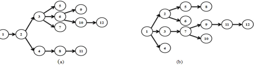
Figure 1: (a), (b) are directed out-tree rooted at node 1

whose elements (nodes) have been numbered from 1 ton and a setE ofm edges(|E| = m). We refer to an undirected edge joining the node pair iandj as {i, j}and a directed one from nodei to nodej as (i, j). Edge(i, j) is an outgoing edge of nodeiand an incoming edge of nodej. Each directed edge(i, j)has an associated cost coefficienttij (in general, tij may not

be equal totji). Also, letP denote the set of all spanning directed paths inG(the paths under

consideration in the ordering problems).

Since any solution of the feasible region in the ordering problem (set P ) is directed (actually, directed spanning path), it is reasonable to work with a directed network as the network under consideration. So, we have the following definition.

Definition 2.1. LetE¯ ={(i, j)and(j, i) :{i, j} ∈E}andG¯ = (N,E¯).

By definition1, each undirected edge {i, j} ∈ E is replaced by two directed edges (i, j)and

(j, i) ∈ E¯, and G¯ is the network obtained from G by this transformation. We recall some terminologies in network flows studied, for example, in combinatorial optimization and then prove a theorem (Theorem 1) that will be of use later.

Definition 2.2. A tree is said to be a directed out-tree rooted at a node if the unique path in the tree from that node to every other node is a directed path (figure1). We show the unique directed path from nodei1 to nodeikby notationi1−i2− · · · −ikand let|p0|denote the length ofp0

(the number of edges inp0) i.e,p0 =|{(i, j)∈E¯: (i, j)∈p0}|.

Also, we say that nodeiis the predecessore of nodej in pathp0, if(i, j)∈p0

Definition 2.3. LetT (includingnnodes numbered from 1 ton) be a directed out-tree rooted at a nodei1 ∈ {1,· · · , n}. IfLidenotes the lable value of nodei, we set,Li1 = 1andLj = 1 +Li

for each(i, j)∈T.

Lemma 2.4. Let T and label values Li(1 = 1,· · · , n) be defined as in definitions 2 and 3.

Suppose thatksdenotes the set of nodes having the same lable value equal tosi.e. ks = {i∈

N :Li =s}. Then,

b)k1 ={i1}

c)1≤Li ≤n,∀i∈N.

d) Ifks=∅, thenkt =∅for eacht ≥s.

e)

n

P

s=1

|ks|=n(|ks|denotes the cardinality ofks).

f)

n

P

s=1

|ks|.s= n

P

i=1

Li

Proof. a) The existence ofp0 is resulted from definition 2. By definition 3, we have Lik = 1 +Lik−1 = 2 +Lik−2 =· · ·= (k−1) +Li1 =|p0|+ 1. SoLik = 1 +|p0|. Ifi1 =ik, p0 is a trivial path consisting of one nodei1 and no edge. Hence,|p0| = 0and we have

Li1 = 1.

b) By definition 3,Li1 = 1that impliesi1 ∈k1. By part (a), for eachik ∈N,Lik = 1 +|p0|.

Ifi1 6=ik, then|p0|>0that impliesLik ≥2. Thus,ik∈/k1.

c) For eachik ∈ N, Lik = |p0|+ 1. Sincep0 has at most n nodes, then p0 ≤ n−1. Thus, 1≤Lik = 1 +|p0| ≤n(ifik=i1,|p0|= 0andLi1 = 1).

d) Since,ks =∅, we have from part (b),s 6= 1. Hence,t ≥s > 1. By contradiction, suppose

that i ∈ kt (i.e. Li = t) and p0 is the unique directed path from i1 toi. If, j1 denotes the predecessor of nodeiin p0, definition 3 impliesLi = 1 + Lj1. Then,Lj1 = t−1.

Similarly, for a nodej2, the predecessor of nodej1, we haveLj1 = 1 +Lj2 that implies

Lj2 =t−2. By repeating, there is a nodejt−swithLjt−s =s, sojt−s∈ksthat contradicts Ks=∅

e) Sinceks ⊆N(s= 1,· · · , n), we have

Sn

s=1ks⊆N. Also, for eachi∈N, we havei∈kLi

(1 ≤ Li ≤ n, from part (c)) that implies N ⊆

Sn

s=1ks. Thus,

Sn

s=1ks = N. From

definitions 2 and 3, ifs 6=t, thenks∩kt=∅. Therefore, n

P

s=1

|ks|=|N|=n.

f) From the proof of part (e),N =Sn

s=1ks andks∩kt=∅, ifs6=t. Hence,

n

X

i=1

Li = n

X

s=1

X

i∈ks Li =

n

X

s=1

(X

i∈ks s) =

n

X

s=1

(S.X

i∈ks 1) =

n

X

s=1

S.|ks|

Lemma 2.5. Let T and label values Li(i = 1,· · · , n) be defined as in definitions 2 and 3. Suppose thatA=

n

P

s=1

ϕ(ks)where

ϕ(ks) =

                  

|k1| P

i=1

i s=1

|ks| P

i=1

(|k1|+|k2|+· · ·+|ks−1|+i) ks 6=∅, s6= 1

0 ks =∅

Then,

a)A= n(n₂+1)

b)Pn

i=1Li ≤Ain which equality holds iff|ks|= 1

Proof. a) From lemma 1 (part (b)),k1 6=∅. We setkn+1 =∅(it is justifiable because|N|=n). Then, without loss of generality, suppose thatt+ 1(t ∈ {1,· · · , n})is the least index such thatkt+1 =∅. So, we have from lemma 1 (part(d)),kt+1 =kt+2 =· · ·=kn =∅.

LetB1 =

t

P

i=1

|ki|andB2 =

n

P

i=t+1

|ki|. Therefore,B2 = 0and

A=Pn

s=1ϕ(ks) =

Pt

s=1ϕ(ks) =

P|k1|

i=1i+

P|k2|

i=1(|k1|+i) +· · ·

P|kt|

i=1(|k1|+· · ·+|kt−1|+i)

= 1 + 2 +· · ·+Pt

i=1|ki|

=PB1

i=1i=

PB1+B2 i=1 i

in which the last equality hold from lemma1 (part(e)).Thus ,A= n(n₂+1)

b) Consider ϕ(ks) (sth term in A). At first, suppose that ks 6= ∅ ands > 1. By definition,

ϕ(ks) = |ks| P

i=1

(|k1|+· · ·+|ks−1|+i). From lemma 1 (part (d)), we have ki 6= ∅, ∀i ∈

{1,2,· · · , s−1}that implies |ki| ≥ 1, ∀i ∈ {1,2,· · ·, s−1}. Hence,s−1 ≤ |k1|+

· · ·+|ks−1|that implies

s ≤ |k1|+· · ·+|ks−1|+i,∀i∈ {1,2,· · · ,|ks|} (*1)

and (*1) is an equality iff|k1| =· · ·=|ks−1|=i= 1. By summing inequalities (*1) for

i= 1,2, ...,|ks|

|ks|.S≤ |ks| X

i=1

Since each side in (*1) is non-negative, (*2) is an equality iff (*1) is an equality for each

i ∈ {1,2,· · · |ks|} iff |k1| = · · · = |ks−1| = |ks| = 1. In special cases, if ks = ∅,

then |ks| = ϕ(ks) = 0, that converts (*2) into trivial equality 0 = 0. Also, if s = 1,

we have, 1 = |k1| =

P|k1|

i=1i = ϕ(k1) in which |k1| = 1, from lemma 1 (part (b)). Therefore, (*2) is true for eachϕ(ks),s= 1,2,· · · , n. By summing inequalities (*2) for

s = 1,2,· · · , n, we havePn

s=1|ks|.s ≤

Pn

s=1ϕ(ks) =Ain which the equality holds iff for eachs ∈ {1,· · · , n}, (*2) is an equality iff for eachs ∈ {1,· · · , n}, eitherks =∅or

|k1|=· · ·=|ks|= 1

Theorem 2.6. LetT and label valuesLi(i= 1,· · · , n)be defined as in definitions 2 and 3. T

is a directed path (fromi1 as the beginning node) iff

n

P

i=1

Li = n(n₂+1).

Proof. At first, we note from definition 2 that ifT is a path, it is a directed path. However, if

T is a directed path, the result follows directly by definition 3. Conversely, suppose that the equality holds. On the contrary, ifT is not a path, there must exist a nodepinT having more than one outgoing edge, say(p, j1),· · ·,(p, jk)∈ T (node 3 in figure 1.a, for example). Thus,

by definition 3, we haveLj1 =· · · =Ljk = 1 +Lp. letLj1 = · · ·=Ljk =q. Since|kq| ≥ 2,

lemma 2 (part(b)) implies

n

P

i=1

Li < n(n_n+1). This contradiction completes the proof.

Definition 4 below introduces the variables of our problem.

Definition 2.7. LetW be a subgragh ofG¯denoted byW ⊆G¯. Set,

xij =

1 if(i, j)∈W

0 otherwise

Equivalently, every variable assignmentxij ∈ {0,1}characterizes a subgraph ofG¯. We write

{i, j} ∈W, if(i, j)∈W or(j, i)∈W. The following lemma gives a useful equivalence.

Lemma 2.8. LetT ⊆G¯be a directed out-tree rooted at a nodei1 ∈ {1,· · · , n}. We set,Li1 = 1

and

Lj−Li ≤(xij −xji) + (n−1)(1−xij −xji) (1)

Lj−Li ≥(xij −xji) + (n−1)(xij +xji−1) (2)

Then, valuesLi(i= 1,· · · , n)are the same as in definition 3.

Proof. Since1≤Li ≤n,∀i∈N (lemma 1, part (c)) we have,−(n−1)≤Lj −Li ≤n−1,

∀i, j ∈ N. By definition 4, xij = xji = 0iff(i, j),(j, i) ∈/ T. In this case, (1) and (2) imply

trivial inequalities−(n−1)≤Lj−Li ≤n−1. By definition 4,(i, j)∈T (and then(j, i)∈/ T)

iff xij = 1 and xji = 0. From (1) and (2), we have Lj −Li = 1 that implies Lj = 1 +Li.

Similarily, definition 4 implies(j, i) ∈ T (and then(i, j) ∈/ T) iffxji = 1 andxij = 0. Thus,

we have from (1) and (2),Lj−Li =−1that meansLi = 1 +Lj. Finally, from definition 3, it

is impossible that(i, j)∈T and(j, i)∈T. However, if we setxij =xji = 1, then (1) , (2) are

For several reasons, we need to extend setsNandE¯by adding an artificial nodesandnartificial directed edges(s, i), i= 1,· · · , n(fromsto every original node) toG¯. Some identities of this new structure are demonstrated by lemma 4 and theorem 2 below required to prove the main theorem of the paper. Other properties ofG∗ will be expressed later in the conclusion section. At first, we present this new structure formally as follows:

Definition 2.9. LetG∗ ={N ∪ {s}, E∗}whereE∗ = ¯E∪ {(s, i) :i= 1,· · ·, n}.

Lemma 2.10. Suppose thatW ⊆G∗ satisfies the following equalities:

X

j∈A(i)∪{s}

xji = 1, i= 1,· · · , n (3)

Where A(i) = {j ∈ N : {i, j} ∈ E}and xsi = 1(xsi = 0) iff(s, i) ∈ W((s, i) ∈/ W), i = 1,· · · , n. Then,

a) eachi∈N is inW (i.e. W is spanning subgraph ofG∗).

b) for each cycleC ⊆W,s /∈C.

c) each cycleC⊆Wis directed.

Proof. a) Leti∈N be an arbitrary node. By (3), there exists the unique nodej ∈A(i)∪ {s}

such thatxji= 1. Now definition 4 implies(j, i)∈W, that meansi∈W.

b) By contradiction, suppose thats ∈ C. LetC be as a sequence of nodesik−ik−1 − · · · −

i1−s−j1−j2− · · · −jk−ik. From definition 5,(j1, s)∈/ C ⊆G∗. Thus, we must have

(s, j1) ∈ C. From (3),(j1, j2) ∈ C. Or else, if(j2, j1) ∈ C. thenj1 has two incoming edges(s, j1)and(j2, j1), and then definition 4 impliesxsj1 =xj2j1 = 1,that contradicts (3)

fori=j1. Using this argument repeatedly, it follows that(j2, j3),(j3.j4),· · · ,(jk−1, jk)

and(jk, ik)∈C. Similarly,(s, i1)∈Cand we have, by repeating the preceding argument,

(i1, i2),(i2, i3),· · · ,(ik−2, ik−1)

and (ik−1, ik) ∈ C. Thus, node ik has two incoming edges (jk, ik) and (ik−1, ik) that

contradicts (3).

c) LetC be as i1−i2− · · · −ir−i1 (s /∈ C, from part (b)). Without loss of generality, let

(i1, i2)∈C. From (3) and definition 4, each nodei∈N must have exactly one incoming edge. Thus, since (i1, i2) ∈ C, we have (i2, i3) ∈ C. Using (3) repeatedly, we have

Theorem 2.11. LetW ⊆ G∗ and variablesLi(i = s,1,· · · , n)be arbitrary (none of them is

pre-specified). IfW satisfies (1),(2) and (3), then W is a spanning directed out-tree rooted at nodes.

Proof. At first, we show thatW has no cycle. By contradiction, suppose that a cycleC ⊆ W. According to lemma 4 (part (c)),C is directed. Hence,C is a directed pathj1 −j2 − · · · −jr

fromj1tojrtogether with(jr, j1). Therefore, (1) and (2) imply thatLj1 < Ljr (because of the

path) andLjr < Lj1 (because(jr, j1)∈C). By this contradiction, the result follows. Now, since W has at leastnnodes as well asnedges (from lemma 4, part (a), and (3)), it must haven+ 1

nodes in the first place (i.e. s ∈ W), and then exactlyn edges in the second place (or else, if each of both cases is not true,W has a cycle). Therefore,W is spanning by the former statement and a tree by the latter. Finally, suppose, by contradiction, that the paths−j1−j2− · · · −jk

inW is not directed. From the definition ofG∗, we have(s, j1) ∈ W. If (j2, j1) ∈ W, then,

j1 contradicts (3). Hence, (j1, j2) ∈ W. In the same manner, we have, (jr−1, jr) ∈ W for

r = 3,4,· · · , k. But, this contradicts, that the path is not directed. Therefore, the unique path inW fromsto every other node is directed. This completes the proof.

Corollary 2.12. LetW = (NW, EW)be a subgraph ofG∗ and satisfy (1),(2),(3) and following

constraints:

n

X

j=1

xsj = 1, Ls= 0 (4)

Ifxsi1 = 1 for some i1 ∈ {1,· · · , n}, thenW¯ = (NW − {s}, EW − {(s, i1)}) is a spanning

directed out-tree rooted at nodei1 inG¯ withLi1 = 1

Proof. From theorem 2, W is a spanning directed out-tree rooted at node s. Hence, W has

n+ 1 nodes(NW = N ∪ {s}) and n edges. From (4), node i1 is only node connected to s withLi1 = 1 +Ls = 1. Thus, by deleting nodesand edge(s, i1),W¯ = (N, EW − {(s, i1)}) is still a connected graph consisting ofnnodes and n−1edges. Therefore, W¯ is a spanning tree inG¯. On the other hand, for an arbitary nodei ∈N, there exists the unique directed path

s−i1−i2− · · · −iinW fromstoi. Thus, by removing nodesand edge(s, i1), i1−i2− · · · −i is the unique directed path inW¯ fromi1to an arbitrary nodei∈N. Therefore,W¯ is a directed out-tree rooted at nodei1. This completes the proof.

The following theorem characterizes the feasible solution set of the ordering problem.

Theorem 2.13. LetW ⊆G∗. IfW satisfies (1),(2),(3),(4) and

n

P

i=1

Li = n(n₂+1), thenW¯ ∈P

Proof. The result follows from corollary1 and Theorem1.

Finally, the objective function of the proposed model is considered as

n

P

j=1

n

P

i=1

tijxij for each

(i, j) ∈ E¯, where the cost coefficients of the artificial edgestsj, j = 1,· · · , n, are equal to 0.

min

n

X

j=1

n

X

i=1

tijxij

for i, j =s,1,· · · , n

Lj −Li ≤(xij −xji) + (n−1)(1−xij −xji)

Lj −Li ≥(xij −xji) + (n−1)(xij +xji−1)

X

j∈A(i)∪{s}

xji = 1 , i= 1,· · · , n

n

X

j=1

xsj = 1, Ls= 0 (5)

n

X

i=1

Li =

n(n+ 1) 2

xij ∈ {0,1} i, j =s,1, ..., n

Remark.

a) It is not necessary, to add a restriction on the outgoing edges of nodes in the problem i.e.

P

j

xij = 1,i =s,1,· · · , n. This constraint is automatically satisfied, as shown in

theo-rems 2 and 3.

b) By theorem 3, the labels of the nodes in a path are ordered from 1 ton. We can find the beginning node of a path simply in two ways; (I) as the node connected to nodes(node

i1, say, for whichxsi1 = 1) or (II) as the node with a label value equal to 1. The end node

of a path is the node with a label value equal ton. Other labels also show the position of the interior nodes in a path.

c) Similar to variablesLi, we can define variablespi(i=s,1,· · · , n)as follows:

ps= 0

pj−pi ≤tij(xij −xji) + (n−1)(1−xij −xji)

pj−pi ≥tij(xij −xji) + (n−1)(xij +xji−1)

It is easy to verify thatpigives actually the time consumed for traveling a path from its beginning

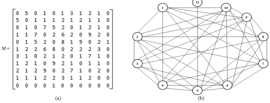
Figure 2: (a) node-node adjacency matrixM = (mi)11×11 in whichmij = tij, (b) undirected

graphG= (N, E)

3 Numerical example

Figure 2.a depicts an undirected graphG = (N, E)with 11 nodes and 41 edges. In figure 2.b,

M = (mij)11×11shows the node-node adjacency matrix ofGwheremij = 0, if{i, j}∈/ Eand

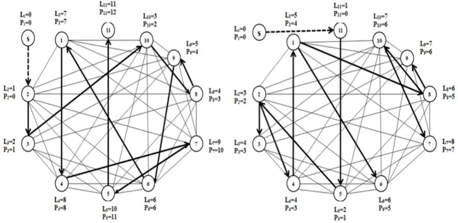
mij =tij ∈E(tij is the cost coefficient of edge{i, j}). Figure 3 depics the minimum spanning

directed path (that is from node 2 to node 11) resulted from theorem 3 with the objective function value 12 and minimum spanning directed out-tree (that is rooted at node 11) characterised by theorem 2 with the objective function value 10 (in figure 3.(b), since the result is a tree, not a path, then the objective function value is not equal to p11). Li ’s are the positions of nodes in

the optimal path. L2 = 1introduces node 2 as the beginning node of the optimum path and

L11 = 11says that node 11 is the end node. Also, for example, L7 = 9shows that node 7 is

9th_{node in the path andp}

8 = 3gives the time of travel from the beginning (node 2) to node 8. Furthermore, we havep2 = 0andp11= 12(total time needed for traveling all of the path)

4 Conclusion

In this section, we present the properties of the proposed model in three subsections.

4.1 Theoretical aspects

Figure 3: (a) Minimum spanning directed path (from node 2 to node 11), (b) Minimum spanning directed out-tree (rooted at node 11)

The properties proved by lemma 4 and theorem 2 can be used in problems in which other optimal structures such as cycles and trees instead of spanning paths are interested to be found.

Similar to nodes, one can add another artificial node t (withLt = n+ 1, if necessary) andn

directed edges(j, t), j = 1,· · · , nfor other special applications.

4.2 Computational aspects

2mvariablesxij for each directed link andnvariablesxsj in order to construct ofG∗. Variables

Li andPi are automatically attained as integer. However, there are several ways to handle such

these situations as stated in the introduction. The model has2m+n+ 2constraints:

2mconstraints by (1) and (2) to find a desired tree (G¯has at leastmcycles for each pair ofxij

andxji).

nconstraints by (3) to find a spanning solution (nnodes must be included).

One constraint by (4) to find a beginning node (each node may play the role of the beginning node in an optimal path).

4.3 Applied aspects

Some problems that can be formulated as this model are presented as follows:

Solving the ordering problem by assuming pre-specified ordering on some nodes in the optimal path. For exampleL4 = 6, L5 = 1, L6 = 2

Solving the ordering problem in which some nodes have to be visited before or after (locally) some others. For exampleL4 ≤L6, L4 ≤L10≤L2

Solving the ordering problem in which the orders of nodes satisfy an special formula (rule). For example,P1 ≤P3+ 4,P11=P3+P5,P2 = 2k+ 1(k ∈N),L3 = 2k,L4+L10 =L2

Solving the ordering problem in which some nodes have to be visited after or before a certain time or in a certain period of time. For exampleP1 ≤5,P3 ≥4,7≤P2 ≤9.

Solving the ordering problem in which some nodes have to be visited befor or after (temporally) some other nodes. For exampleP3 ≥P4

Finding the shortest path emanating from a certain nodei0: we set initially,Li0 = 1, in problem

(5)

Finding the shortest path terminating at the certain nodei0: we set initially,Li0 =n, in problem

(5)

Finding the shortest path from a certain nodei0 to a certain nodei1 such that nodei2 is in the middle of the path. For example, ifnis an even number, we setLi0 = 1,Li1 =n,Li2 = n₂.

Finding the shortest path with certain length or cost equal to R0 from nodei0 to nodei1. We add the following constraints in problem (5):

X

j

X

i

cijxij =R0

Li0 = 1, Li1 =n

5 Acknowledgement

This work was supported by Tehran University. Our special thanks go to the University of Tehran, College of Engineering and Department of Engineering Science for providing all the necessary facilities available to us for successfully conducting this research.

References

[1] Ausiello, P. Crescenzi, G. Gambosi, V. Kann, A. Marchetti-Spaccamela, and M. Protasi., Complexity and approximation . Springer-Verlag, Berlin, 1999.

[3] Barenholz, U. Feige, U., Peleg, D.: Improved approximation for min-sum vertex cover. (2006)

[4] Bar-Yehuda, R. Even, G., Feldman, J., and Naor, J. Computing an optimal orientation of a balanced decomposition tree for linear arrangement problems. Journal of Graph Algorithms and Applications 5, 4, 1-27. 2001.

[5] Bazarra, M. S. Jarvis, J., Sherali, H. D., Linear programming and network flows, Third Edition, Published Online: 15 AUG 2011.

[6] Becker, O. : Das Helmstädtersche Reihenfolgeproblem - die Effizienz verschiedener Näherungsverfahren, in Computer Uses in the Social Science, Wien, January 1967.

[7] Campos, V. Glover, F., Laguna, M. and Martí, R.: An experimental evaluation of a scatter search for the linear ordering problem , J. Global Optim. 21(4), 397-414, 2001.

[8] Campos, V. Laguna, M. and Martí, R.: Scatter search for the linear ordering problem, in D. Corne, M. Dorigo and F. Glover (eds), New Ideas in Optimization, McGraw-Hill, London, UK, pp. 331-339. 1999.

[9] Chanas, S.and Kobylanski, P.: A new heuristic algorithm solving the linear ordering problem , Comput. Optim. Appl. 6 , 191-205, 1996.

[10] Charikar, M. Hajiaghayi, T., Karlo, H., and Rao, S. B., 22 spreading metrics for ordering problems. To appear, SODA, 2006.

[11] Chekuri, C., Ene, A.: Approximation algorithms for submodular multiway parti- tion. In: Proceedings of the 2011 IEEE 52nd Annual Symposium on Foundations of Computer Science. FOCS ’11, Washington, DC, USA, IEEE Computer Society .807-816 . 2011.

[12] Congram, R. K.: Polynomially searchable exponential neighbourhoods for sequencing problems in combinatorial optimisation, PhD thesis, University of Southampton, Faculty of Mathematical Studies, UK, 2000.

[13] Corso, G. M. D. and Romani, F. Heuristic spectral techniques for the reduction of bandwidth and work-bound of sparse matrices. Numerical Algorithms 28, 1-4 (Dec.), 117-136. 2001a.

[14] Devanur, N.R., Khot, S.A., Saket, R., Vishnoi, N.K.: Integrality gaps for sparsest cut and minimum linear arrangement problems. In: Proceedings of the 38th Annual ACM Symposium on Theory of Computing. STOC ’06, New York, NY, USA, ACM . 537-546, 2006.

[15] Even, J. Naor, S. Rao, and B. Schieber. âŁœDivide-and-conquer approximation algo-rithms via spreading metrics⣞. In 36th IEEE Symposium on Foundations of Computer Science,pages 62⣓71, 1995.

[17] Feige, U., Lov-asz, L., Tetali, P. Approximating min sum set cover. Algorithmica 40 . 219-234 . 2004.

[18] Garey, M. R., Johnson, D. S. Computers and Intractability. A guide to the theory of NP-completeness. Freeman and Company, 1979.

[19] M. R. Garey, D. S. Johnson, and L. Stockmeyer. Some simplified NP-complete graph problems. Theoretical Computer Science, 1:237-267, 1976.

[20] Goel, G., Karande, C., Tripathi, P., Wang, L.: Approximability of combinatorial problems with multi-agent submodular cost functions. In: Proceedings of the 50th Annual IEEE Symposium on Foundations of Computer Science. FOCS ’09, Washington, DC, USA, IEEE Computer Society . 755-764. 2009.

[21] Grötschel, M. Padberg, MW: Polyhedral aspects of the Traveling Salesman Problem I. Theory, European Institute for Advanced Studies in Management. W. Germany. 1983a.

[22] Grötschel, M. Padberg, MW: Polyhedral aspects of the Traveling Salesman Problem II. Computation., European Institute for Advanced Studies in Management. W. Germany. 1983b.

[23] Grötschel, M: Approaches to Hard Combinatorial Optimization Problem, in Korte, B (ed) : Modern Applied Mathematics: Optimization and Operations Research, North-Holland Publishing Co. Amsterdam - New York -. Oxford, 437-575, 1982.

[24] Grötschel, M., Jünger, M. and Reinelt, G.: A cutting plane algorithm for the linear ordering problem, Oper. Res. 32(6), 1195-1220, 1984.

[25] Hansen, M., Approximation algorithms for geometric embeddings in the plane with ap-plications to parallel processing problems, in Proceedings of the 30th Annual Symposium on Foundations of Computer Science, IEEE Computer Society Press, Los Alamitos, CA, pp.604-609, 1989.

[26] Hu, Y. F. and Scott, J. A. A multilevel algorithm for wavefront reduction. SIAM J. Sci. Comput. 23, 4, 1352-1375. 2001.

[27] Ilya Safro. Dorit Ron. Achi Brandt : Multilevel Algorithms for Linear Ordering Problems, The Weizmann Institute of Science . 2009.

[28] Iwata, S., Nagano, K.: Submodular function minimization under covering con- straints. In: Proceedings of the 50th Annual IEEE Symposium on Foundations of Computer Science. FOCS ’09, Washington, DC, USA, IEEE Computer Society . 671-680. 2009.

[29] Juvan, M. Mohar, B., Optimal linear labeling and eigenvalues of graphs. Discrete Applied Mathematics, 36(2):153-168, 1992.

[31] Laguna, M., Martí, R. Campos, V.: Intensification and diversification with elite tabu search solutions for the linear ordering problem, Comput. Oper. Res. 26(12) , 1217-1230. 1999.

[32] Leighton, F. T. Rao, S. Multicommodity max-flow min-cut theorems and their use in designing approximation algorithms, J. ACM, 46, pp. 787-832, 1999.

[33] Liu, W. Vannelli, A. Generating lower bounds for the linear arrangement problem. Discrete Applied Mathematics, 59:137-151, 1995.

[34] Mitchell, J. E. and Borchers, B.: Solving linear ordering problems with a combined interior point/simplex cutting plane algorithm, in H. L. Frenk, K. Roos, T. Terlaky and S. Zhang (eds), High Performance Optimization, Kluwer Academic Publishers, Dordrecht, The Netherlands, pp. 349-366. 2000.

[35] Mushi, A.R : The Linear Ordering Problem: An Algorithm for the optimal solution, Mathe-matics Department, University of Dar es salaam. African Journal of Science and Technology (AJST) Science and Engineering Series Vol. 6, No. 1, pp. 51-64.

[36] Petit, J. Experiments on the minimum linear arrangement problem. ACM Journal of Ex-perimental Algorithmics, 8. 2003.

[37] Rao, S. Richa, A. W., New approximation techniques for some linear ordering problems. SIAM J. Comput. 34(2):388-404, 2004.

[38] Ravi, R. Agrawal, A. Klein, P., Ordering problems approximated: Single-processor scheduling and interval graph completion, in Proceedings of the 18th International Col-loquium on Automata, Languages, and Programming, Lecture Notes in Comput. Sci. 510, Springer-Verlag, Berlin, pp. 751-762, 1991.

[39] Safronetz, D., R. Lindsay, B. Hjelle, R. A. Medina, K. Mirowsky-Garcia, and M. A. Drebot. Use of IgG avidity to indirectly monitor epizootic transmission of Sin Nombre virus in deer mice (Peromyscus maniculatus). American Journal of Tropical Medicine and Hygiene 75: 1135-1139 . 2006.

[40] Satoru Iwata (Research Institute for Mathematical Sciences, Kyoto University), Prasad Tetali (School of Mathematics, Georgia Institute of Technology) , and Pushkar Tripathi (School of Computer Science, Georgia Institute of Technology) : Approximating Minimum Linear Ordering Problems. 2013

[41] Schiavinotto, T. and Stützle, T.: Search space analysis of the linear ordering problem, in G. R. Raidl et al. (eds), Applications of Evolutionary Computing, Lecture Notes in Comput. Sci. 2611, Springer-Verlag, Berlin, pp. 322-333. 2003.