Telephone: +44 (0)1582 763133 Web: http://www.rothamsted.ac.uk/
Rothamsted Research is a Company Limited by Guarantee Registered Office: as above. Registered in England No. 2393175. Registered Charity No. 802038. VAT No. 197 4201 51. Founded in 1843 by John Bennet Lawes.
Rothamsted Repository Download
A - Papers appearing in refereed journals
Gower, J. C. 1968. Adding a point to vector diagrams in multivariate
analysis. Biometrika. 55 (3), pp. 582-585.
The publisher's version can be accessed at:
•
https://dx.doi.org/10.1093/biomet/55.3.582
The output can be accessed at:
https://repository.rothamsted.ac.uk/item/8w1vz
.
© Please contact [email protected] for copyright queries.
Adding a point to vector diagrams in multlvariate analysis
BY J. C. GOWER
Rothamsttd Experimental Station
STJMMABY
A set of n base points P{ (i = 1,2, ...,n), with known co-ordinates relative to orthogonal axes, and a further point P.+ 1, with known distance from each of the base set, are given. The co-ordinates of P»+l
relative to the axes of the base set are found. The formula is particularly simple when the base set is referred to its principal axes, when the co-ordinates otPn+1 for a subset of all the axes can be calculated from the co-ordinates of the P{ in this subset only. The classical results for adding a point to a principal components or canonical variates analyses are obtained when the base set is derived using the appro-priate distance functions. An example ifl given.
1. DERIVATION or THE BASIC FOBMXTLA
Gower (1966a) discussed how the co-ordinates of n points -P<(t = 1,2, ...,n) referred to principal axes can be found, given the Euclidean distances dtl between all point pairs Pt and Pt; principal components and canonical variate analysis are special cases. The points are supposed to he in an wi-dimensional space; normally m = n— 1 but in exceptional cases m can be lees. The successive steps in this method may be summarized as follows:
(i) define the matrix A whose elements are — JdJ^; (ii) define B with elements b(l = au — ai—aj + a;
(iii) find the m non-zero latent roots A = diag(A!, A,,..., A^,) of B and corresponding vectors X standardized so that X'X = A. Thus BX = XA and
X X ' = B. (1)
The tth row of X gives the co-ordinates (xtl,xi%, ...,xim) of P(; the points are centred so that the origin is at the centroid O, i.e. the column sums of X are zero. When B is not positive semi-definite some values of A, will be negative and all co-ordinate values along the corresponding axes will have imaginary values. In this case the distances cannot be Euclidean but the results given here remain valid if we accept imaginary values in the usual distance formula djy = (xtl — xn)% +... + {xin — xjm)*.
The tth diagonal element of XX' may be written xjj +... + xjm; this is the square of the distance d{ of
Pt from the centroid, and therefore from (1)
bu = d« (2)
a result which will be needed later. The geometrical interpretation of the off-diagonal elements of B is that bu = didjcosdij, where 6tj is the angle subtended by the line PtPjat the centroid, but this result will not be needed here.
When a further point becomes available, a method is needed for finding its co-ordinates
" » + l (xn+\, If * « + l , !>•••>+\, If * « + l , !>•••> x xn+\, m>n+\, m> x xn+l. m + l )n+l. m + l
relative to the axes used for the P< (t < n), allowing for an (m+ l)th dimension which may bo needed to represent exactly all the new given distances df ,+ x (t = 1,2, ...,n). The co-ordinates can be found by
solving the n quadratic equations
m+l
< * ! . + ! = £ ( * . « , *-*«,*)• ( i = 1.2 n ) (3)
fc-l
where xim+1 = 0 when i 4= n+ 1.
Before showing how the equations (3) can be conveniently solved, a few remarks are appropriate. In principal component analyses the point Pn+1 will not need an extra dimension for its representation, unless m happens to be less than the total number of variates in the analysis, and the distances d(t n+1 can be readily computed from the data. Because xn+1 t is the orthogonal projection of Pn+1 onto the
kth axis, the solution of (3) using these distances must agree with the classical method for adding a point
in a principal components analysis; similar remarks apply to canonical variate analysis. This result, obvious geometrically, is verified below algebraically. Although m will alwayB be less than n so that some of the n equations in (3) must be redundant, it is evident from the geometrical derivation that these
equations are consistent. For example, if n = 10 and m = 1 so that the base set consists of 10 collinear
points, Pn is fixed by two distances, say d^ u and du n, but the remaining 8 distances will be consistent
with these two. Even in the worst case there are enough equations to find all m+ 1 co-ordinates of
Pn+1, for then the n base points will require n — 1 dimensions for their representation so that m + 1 ^ n.
To solve (3), the equations will first be written in the alternative form
C i = il.+i + (? -2S % V i . t ( i = l,2,...,n). (4)
Because of the centring, the cross-product term in (4) vanishes when these equations are summed over t. Thus
2 <*?..+i = ™S+i+ 2 < S . (5)
i - l i-1
which can be used to substitute for djj+1 in (4), giving after a little rearrangement
2 S * « * = < * ? - < * ! j (dj-tfj + l) . (6)
fc-l ni - l
This is a set of n linear equations in the m unknowns xn+ltk (k = 1,2, ...,m). These equations are
con-sistent because they have been derived by linear operations from the set of concon-sistent equations (3). As all the distances on the right-hand side of (6) are known, the first m equations may be solved to find the required values, but a more symmetric method is convenient. First putting (6) into matrix form by
defining x ' to be the 1 x m vector (xn+1_ lf xn+lt „ ..., xn+li m), d to be the n x l vector whose ith element is
dj — dj n+1 and U to be the nxn matrix all of whose elements are units, we have that
2Xx = d - - U d . (7)
Hence on pre-multiplying both sides of (7) by X', and noting that XTJ = 0 because of the centring, and inverting, it follows that
x=4<X'X)-1X'd. (8)
This is a symmetric form of the solution to (7) and gives the co-ordinates of PB+1 in the first m dimensions,
the value of x,+i>m+1 is conveniently obtained by calculating dn+1 from (5) and using
m
»i+i.«+i = ^ + i - S "i+i,*- (»)
Thus the first m co-ordinates are uniquely defined but the (m + l)th is determined in value but not sign. So far the principal axis property of x has not been used; the results (8) and (9) are applicable to any centred base set X referred to orthogonal axes. When X is referred to principal axes (8) becomes
x = |A-!X'd. (10)
Because A is diagonal, the value of xn+1 t is determined solely from At, the ifcth column of X and the
elements of d. The quantities dj occurring in d are diagonal elements of XX' and their evaluation would seem to need all the columns of X but it was shown in (1) that XX' = B, a matrix whose elements are simply computed and which is in any case needed to compute even only one column of X. Thus if the
analysis leading to (1) is used to give a representation of the base-set of points P{ in r (< m) dimensions,
e.g. by ignoring axes with small At, (10) can still be used to find the co-ordinates of the projections of
PH+1 on to the reduced space using only r columns of X, the known true distances df of P<(i = 1, 2, ...,n)
from their centroid, obtained from the matrix B, and the known true distances df n+1. The residual
distance dn+UroiPn+1 from the r-dimensional plane is then given by a modification of equation (9) and is
k — 1
When the co-ordinates of the base-set are not referred to principal axes formula (8) must be used, and
this requires all m columns of X to compute (X'X)-1.
2. PBTNCIPAL COMPONENT AND CANONICAL VABIATE ANALYSIS
A simple geometrical argument has shown that (10) must reduce to the deaired results when adding a point in a principal components or canonical variates analysis. This is not obvious from an inspection of (10) but is readily verified algebraically.
In a canonical variates analysis on n populations with v measured variates and common dispersion matrix W, the means for the »th population will be written as the l x o vector g4 (t = 1,2,..., n). The
n x t matrix G of all the population means has rows g( and is supposed centred so that the column sums,
ignoring any differences in population sizes, are zero. The latent roots A and vectors L satisfying
G'GL = WLA (12)
can be found and the population means referred to canonical variate axes are denned by
X = GL, (13)
where the vectors are normalized so that L'WL = I. Reasons for sometimes using G'G rather than the usual weighted between-population dispersion matrix were discussed by Gower (1966 6). The co-ordinates X of the base set are defined by (13) and the usual formula giving the co-ordinates x(t> x 1) referred to the canonical axes of a new sample g(lxv) referred to the original variate axes is
x = L'g'. (14)
Mahalanobis's D1 is the appropriate distance for this type of analysis and therefore
<£+M = ( g - g < ) W - i ( g - g , ) ' and d* = &W-%. (15)
Therefore cZJ - d j+ 1 >, = 2 g , W -1g ' - g W -1g ' and d = 2 G W -1g ' - g W1g ' l , (16)
where 1' is an n x 1 vector of unite. Insertion of these results in (10) gives
iA-!X'd = JA-1L'G'(2GW-1g'-gW-1g'l). (17)
The second term on the right-hand side of (17) vanishes because G'l = 0 so that
which simplifies by using the transpose of (12) to
iA-!X'd = A-1AL'WW-1g' = L'g', (18)
agreeing with (14) as required.
The verification for principal components is almost identical, but with W replaced by I, and G interpreted as a n x v data matrix derived from observations on v variates for a multivariate sample of size n.
3 . TflTTAArPT.TH
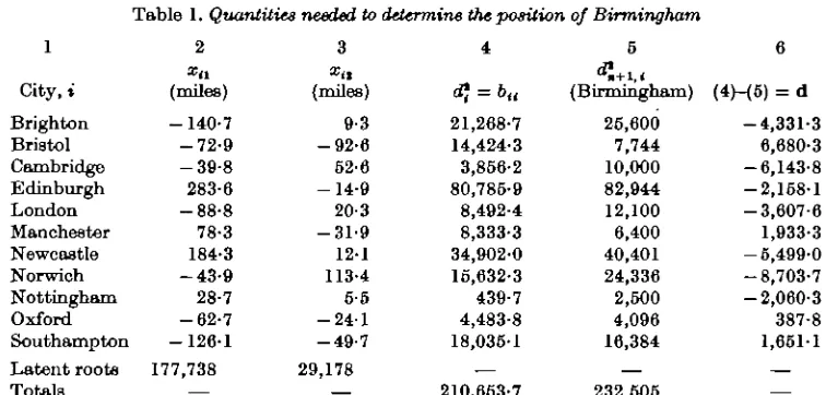
Columns 2, 3 and 4 of Table 1 were derived from a table giving the distances dtj between every pair of eleven British cities, using the method described by Gower (1966 a) and outlined here in the discussion leading to (1) and (2). These constitute the calculations needed to find the co-ordinates of the base-set, here in two dimensions, and remain fixed when positioning a new city. The third, fourth and fifth roots are 6878, 2338 and 288, all arrmll compared with the first two, given in Table 1, and the five remaining roots are negative with a total value of — 6966, less in modulus than A,. Therefore, although an exact reproduction of the given distances is impossible in two dimensions, or in any number of real dimensions, these co-ordinates give quite a good Euclidean representation of the relative positions of the cities; the road distances as reproduced are, on the average, about 1-13 times the direct distanoes.
The squared distances dj+ 1 , of a further city, Birmingham, from each city of the base set are given
in column 6 and the elements of the vector d, found by subtracting column 5 from 4, are given in column 6. The latent roots A1 and A, found in the base set analysis are required and it can be checked from Table 1 that
11 n
Ax = 2 ai and A, = £ *?,.
f - 1 i-1
The first co-ordinate a ^ x of Birmingham is found as the sum of products of columns (2) and (6) divided
by 2AX; this gives
*i*. 1 = - 69,6384-26/(2 x 177,738) = - 2-0.
Similarly, a ^ , = - 2,241,066/(2 x 29,178) = - 38-4.
The position (— 2-0, — 38-4) places Birmingham very well. Its distance d\t from the centroid of the base
set is found from equation (5) as
lid*, = 232,505-210,653-7 = 21,851-3.
Table 1. Quantities needed to determine the position of Birmingham
City, i Brighton Bristol Cambridge Edinburgh London Manchester Newcastle Norwich Nottingham Oxford Southampton Latent roots Totals (miles) -140-7 -72-9 -39-8 283-6 -88-8 78-3 184-3 -43-9 28-7 -62-7 -126-1 177,738 (miles) 9-3 -92-6 52-6 -14-9 20-3 -31-9 12-1 113-4 5-5 - 2 4 1 -49-7 29,178
*(=bti
21,268-7 14,424-3 3,856-2 80,785-9 8,492-4 8,333-3 34,902-0 15,632-3 439-7 4,483-8 18,035-1 — 210,653-7 (Birmingham) 25,600 7,744 10,000 82,944 12,100 6,400 40,401 24,336 2,500 4,096 16,384 232,505
(4H5) = d
-4,331-3 6,680-3 -6,143-8 -2,158-1 -3,607-6 1,933-3 -5,499-0 -8,703-7 -2,060-3 387-8 1,661-1
Columns 1,2,3 and 4 are given by the calculations for the base-set and are determined in a preliminary analysis. Column 5 is given and 6 is the difference between 4 and 5.
Thus dj, = 1986-5, i.e. minus the mean of column 6 and the residual distance l i ^ , of Birmingham from the plane of the base set is found from equation (11) to be 22-5 miles. It must be remembered that
this residual has real and imaginary components so that dj, r may become small because of the possible
cancellation of large positive and negative components; this would not be so if the original distances had been Euclidean giving no negative latent roots. In this example the root-mean-square residual of the base set in the direction of the third dimension is (6878/11)* = 25-0 miles and the total root-mean-square residual out of the fitted plane, using positive and negative roots, is (3538/11 )* = 17-9 miles, both agreeing
well with dlt r. However, a critical examination of this residual would require the real and imaginary
components, separately.
A glance at an atlas reveals that Birmingham is well within the region covered by the base set and the usual warnings apply to extrapolation outside this region; the position of John O'Groats would be poorly determined with the base set chosen here.
REFERENCES
GOWEB, J. C. (1966a). Some distance properties of latent root and vector methods used in multi-variate analysis. Biometrika 53, 325-38.
GOWEB, J. C. (19666). A Q-technique for the calculation of canonical variates. Biometrika 53, 588-9.
[Received February 1968. Revised April 1968]