in the population sciences published by the Max Planck Institute for Demographic Research Doberaner Strasse 114 · D-18057 Rostock · GERMANY www.demographic-research.org
DEMOGRAPHIC RESEARCH
VOLUME 6, ARTICLE 17, PAGES 469-486
PUBLISHED 28 JUNE 2002
www.demographic-research.org/Volumes/Vol6/17/
DOI: 10.4054/DemRes.2002.6.17
Seasonality of Deaths in the U.S. by Age
and Cause
Craig A. Feinstein
1 Introduction 470 2 Analysis of seasonality by age and cause using
NCHS data
470
3 Variation of seasonality of deaths with respect to age
478
4 Seasonality over the years 482
5 Acknowledgements 485
Seasonality of Deaths in the U.S. by Age and Cause
Craig A. Feinstein1
Abstract
In this paper, we analyze seasonality of deaths by age and cause in the U.S. using public use files for the years 1994 to 1998 by the methods of regression and a variation of Census Method II. We answer the following questions: For each age cohort, how much does each cause of death contribute to seasonality of deaths? What is the reason for the variation in seasonality of deaths with respect to age? We also analyze death records of Social Security Administration over a longer time period to examine how seasonality of deaths has changed since the mid-1970’s. We found that in general, the degree of seasonality in deaths has decreased over time for younger cohorts and has increased over time for older cohorts.
1 U.S. Social Security Administration
1. Introduction
It is a known fact that in the U.S., the overall death rates are higher in the winter months than they are at other times of the year. However, there is little current research on this phenomenon. The most recent analysis done in the U.S. that we could find on this topic was a paper by Seretakis et al. (1997) which discussed the seasonality of mortality for coronary heart disease in the U.S. from 1937 through 1991. Earlier, Rogot, Fabsitz, and Feinleib (1976) used U.S. National Center for Health Statistics data from 1962 to 1966 to analyze seasonal patterns with respect to different causes of deaths, including determining correlations between different causes. And Rosenwaike (1966) utilized the “Census Method II” procedure to analyze the seasonality of U.S. deaths from 1951 to 1960 with respect to different causes.
In this note, we analyze the seasonality of mortality for subsets of deaths distinguished not only by cause but also by age of decedent, using death certificate data obtained from the National Center for Health Statistics for the years 1994 to 1998. We also examine why seasonality is more prevalent in certain age groups by observing cause-seasonalities of death and distributions in causes of death with respect to age. Furthermore, using Social Security’s SSI records and the death file of the Office of the Chief Actuary at the Social Security Administration from 1976 to 1999, we observe how seasonal variation in mortality has changed over the years, and whether it varies by poverty status.
2. Analysis of Seasonality by Age and Cause Using NCHS Data
We obtained from the NCHS CD-ROM information on everyone that died in the years 1994 to 1998, and tabulated the number of deaths in each of the sixty months within the five-year period by age group and cause. Because some months have more days than
others do, we computed a(t), the average number of deaths per day in month t for each
Table 1: Average Number of Deaths per Day by Age Group and Cause over the Five Year Period
Cardio-vascular Dia-betes Diges-tive External Causes Infections Parasitic Kidney Malignant Neoplasm Respi-ratory Other All Causes
0 to 4 3 0 0 11 3 0 1 2 76 96
5 to 9 0 0 0 5 1 0 1 0 3 10
10 to 14 1 0 0 7 0 0 1 0 3 12
15 to 19 1 0 0 32 1 0 2 1 4 41
20 to 24 2 0 0 38 2 0 3 1 5 51
25 to 29 4 1 0 34 7 0 4 1 6 57
30 to 34 8 1 1 36 17 0 9 2 10 84
35 to 39 17 2 4 38 21 1 17 3 14 117
40 to 44 30 3 7 34 20 1 30 4 18 147
45 to 49 48 5 8 27 14 1 49 5 21 178
50 to 54 67 7 8 20 9 1 73 8 21 214
55 to 59 90 9 8 16 7 2 100 13 24 269
60 to 64 133 13 8 14 7 3 140 24 32 374
65 to 69 201 19 9 15 9 5 197 44 48 547
70 to 74 295 25 10 18 11 8 241 69 72 749
75 to 79 379 27 8 20 13 10 233 89 100 879
80 to 84 446 25 6 20 13 12 190 97 125 934
85 to 89 428 18 4 17 12 11 119 84 125 818
90 to 94 293 9 2 10 7 7 51 53 86 518
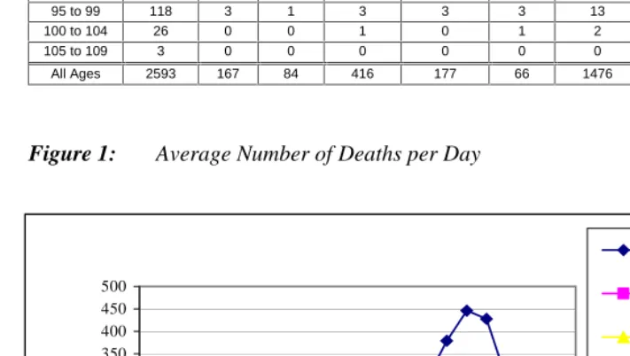
95 to 99 118 3 1 3 3 3 13 21 35 200
100 to 104 26 0 0 1 0 1 2 5 8 43
105 to 109 3 0 0 0 0 0 0 1 1 5
All Ages 2593 167 84 416 177 66 1476 527 837 6343
Figure 1: Average Number of Deaths per Day
0 50 100 150 200 250 300 350 400 450 500
0 10 20 30 40 50 60 70 80 90
Using the “X-11 Variation of Census Method II”, a modification of “Census Method II”, we measured seasonality of deaths. This procedure is an elaboration of a
moving-average method: First, a centered, 12-term moving moving-average c(t)is applied toa(t). The
algorithm proceeds by attempting to improve the estimation of the seasonal component, )
(t
a /c(t), by smoothing the irregular components and extreme values to obtain s(t).
Ifs(t)was not significant at the 1% level, we sets(t)= 1. We defined seasonality as
s = [max t=1,2,...,12 {
∑
− = + 1 0 ) 12 ( n k k t
s }/min t=1,2,...,12{
∑
− = + 1 0 ) 12 ( n k k t
s }] – 1
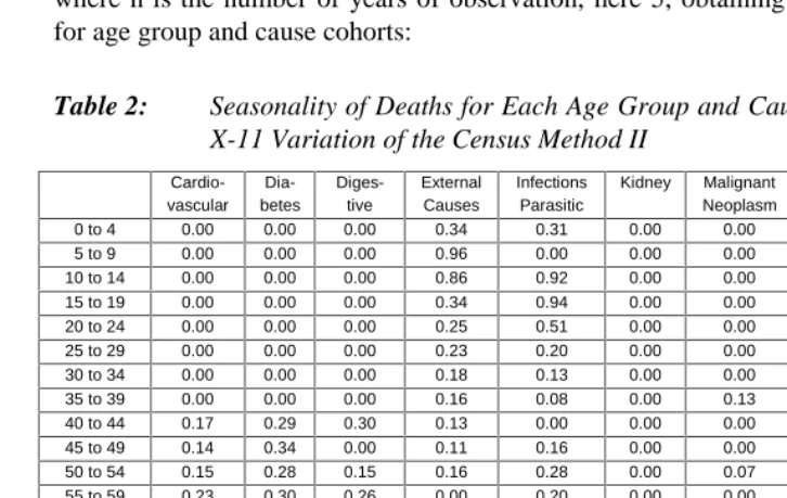
where n is the number of years of observation, here 5, obtaining the following results for age group and cause cohorts:
Table 2: Seasonality of Deaths for Each Age Group and Cause Cohort, Using the X-11 Variation of the Census Method II
Cardio-vascular Dia-betes Diges-tive External Causes Infections Parasitic Kidney Malignant Neoplasm Respi-ratory Other All Causes
0 to 4 0.00 0.00 0.00 0.34 0.31 0.00 0.00 1.88 0.10 0.07
5 to 9 0.00 0.00 0.00 0.96 0.00 0.00 0.00 1.21 0.52 0.39
10 to 14 0.00 0.00 0.00 0.86 0.92 0.00 0.00 0.00 0.27 0.34
15 to 19 0.00 0.00 0.00 0.34 0.94 0.00 0.00 0.00 0.00 0.22
20 to 24 0.00 0.00 0.00 0.25 0.51 0.00 0.00 0.76 0.26 0.16
25 to 29 0.00 0.00 0.00 0.23 0.20 0.00 0.00 0.53 0.19 0.12
30 to 34 0.00 0.00 0.00 0.18 0.13 0.00 0.00 0.78 0.00 0.07
35 to 39 0.00 0.00 0.00 0.16 0.08 0.00 0.13 0.92 0.19 0.07
40 to 44 0.17 0.29 0.30 0.13 0.00 0.00 0.00 0.90 0.18 0.08
45 to 49 0.14 0.34 0.00 0.11 0.16 0.00 0.00 0.75 0.12 0.09
50 to 54 0.15 0.28 0.15 0.16 0.28 0.00 0.07 0.74 0.17 0.13
55 to 59 0.23 0.30 0.26 0.00 0.20 0.00 0.00 0.76 0.19 0.14
60 to 64 0.23 0.25 0.22 0.12 0.26 0.00 0.05 0.79 0.25 0.17
65 to 69 0.25 0.23 0.19 0.00 0.25 0.25 0.04 0.79 0.26 0.20
70 to 74 0.29 0.23 0.20 0.09 0.30 0.32 0.04 0.74 0.29 0.22
75 to 79 0.31 0.27 0.30 0.00 0.41 0.30 0.06 0.83 0.31 0.27
80 to 84 0.34 0.31 0.25 0.24 0.44 0.42 0.08 0.92 0.37 0.33
85 to 89 0.36 0.31 0.32 0.26 0.58 0.47 0.09 1.10 0.41 0.39
90 to 94 0.39 0.35 0.31 0.38 0.51 0.42 0.10 1.22 0.43 0.42
95 to 99 0.39 0.67 0.00 0.42 0.79 0.45 0.16 1.47 0.52 0.50
100 to 104 0.45 0.00 0.00 0.00 0.94 0.00 0.39 1.14 0.60 0.48
105 to 109 0.58 0.00 0.00 0.00 0.00 0.00 0.00 1.57 0.00 0.63
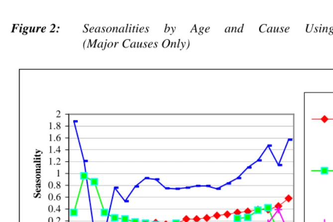
Figure 2: Seasonalities by Age and Cause Using the X-11 Method (Major Causes Only)
A paper by Mackenbach, Kunst, and Looman entitled “Seasonal variation in mortality in The Netherlands” (1992) describes another procedure which measures seasonality in deaths by utilizing non-linear regression. Using this procedure, for each age group and cause, we performed a least squares fit with the equation,
), ( log ) (
loga t = m+β t−t0
where a(t) is the average number of deaths per day in month t, m is the average
number of deaths per day for the five year period, and t0 is the midpoint between the
start of 1994 and the end of 1998. We added a term to measure seasonality to the equation, and using the Levenberg-Marquardt algorithm on the software package
SAS, we performed another least squares fit using:
)) ( 2 cos( )
( log ) (
loga t = m+β t−t0 +γ1 π t−τ1
If the added term was not statistically significant at a 1% level (using analysis of variance with the F-test), we assumed that there was negligible seasonality of deaths present in the cohort. But if the added term was significant, we assumed that there was seasonality present in the cohort, and we subsequently added the
0 0.2 0.4 0.6 0.8 1 1.2 1.4 1.6 1.8 2
0 10 20 30 40 50 60 70 80 90
100
Age
S
eas
on
alit
y
Cardiovascular
External Causes
Malignant Neoplasm
termsγkcos(2π⋅k⋅(t−τk)) where k=2, 3, etc. to the equation until k = 5 or in which the added term was not statistically significant at a 1% level. We computed the maximum and minimum with respect to time of the expression,
))] ( 2 cos( exp[
) (
1
k n
k
k t
t
s =
∑
γ ⋅ π −τ =(where n is the number of added cosine terms) which is an estimate of the seasonal component of the estimated number of deaths per day in each month, t. We define
seasonality as s = [maxs(t)/mins(t)] – 1. Table 3 and Figure 3 display the seasonality
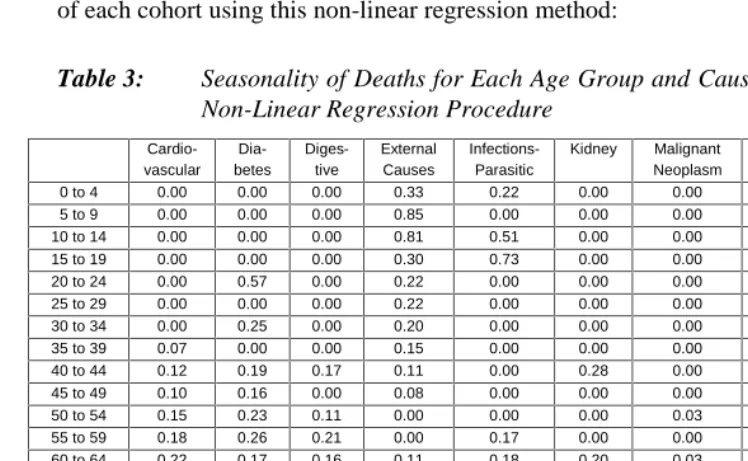
of each cohort using this non-linear regression method:
Table 3: Seasonality of Deaths for Each Age Group and Cause Cohort, Using the Non-Linear Regression Procedure
Cardio-vascular
Dia-betes
Diges-tive
External Causes
Infections-Parasitic
Kidney Malignant Neoplasm
Respi-ratory
Other All Causes
0 to 4 0.00 0.00 0.00 0.33 0.22 0.00 0.00 1.72 0.06 0.05
5 to 9 0.00 0.00 0.00 0.85 0.00 0.00 0.00 0.91 0.30 0.34
10 to 14 0.00 0.00 0.00 0.81 0.51 0.00 0.00 0.00 0.21 0.32
15 to 19 0.00 0.00 0.00 0.30 0.73 0.00 0.00 0.00 0.14 0.22
20 to 24 0.00 0.57 0.00 0.22 0.00 0.00 0.00 0.44 0.00 0.16
25 to 29 0.00 0.00 0.00 0.22 0.00 0.00 0.00 0.29 0.13 0.11
30 to 34 0.00 0.25 0.00 0.20 0.00 0.00 0.00 0.51 0.00 0.00
35 to 39 0.07 0.00 0.00 0.15 0.00 0.00 0.00 0.59 0.08 0.00
40 to 44 0.12 0.19 0.17 0.11 0.00 0.28 0.00 0.68 0.11 0.04
45 to 49 0.10 0.16 0.00 0.08 0.00 0.00 0.00 0.59 0.08 0.08
50 to 54 0.15 0.23 0.11 0.00 0.00 0.00 0.03 0.68 0.15 0.10
55 to 59 0.18 0.26 0.21 0.00 0.17 0.00 0.00 0.69 0.20 0.13
60 to 64 0.22 0.17 0.16 0.11 0.18 0.20 0.03 0.73 0.19 0.15
65 to 69 0.22 0.20 0.14 0.00 0.17 0.17 0.03 0.65 0.20 0.16
70 to 74 0.25 0.20 0.17 0.12 0.24 0.22 0.03 0.64 0.24 0.19
75 to 79 0.27 0.23 0.24 0.05 0.32 0.27 0.04 0.68 0.27 0.23
80 to 84 0.30 0.25 0.13 0.14 0.33 0.32 0.05 0.74 0.33 0.28
85 to 89 0.32 0.27 0.22 0.21 0.42 0.38 0.07 0.83 0.36 0.33
90 to 94 0.33 0.29 0.23 0.29 0.40 0.35 0.08 0.95 0.38 0.36
95 to 99 0.34 0.38 0.30 0.27 0.49 0.38 0.12 1.05 0.43 0.40
100 to 104 0.39 0.00 0.00 0.46 0.00 0.00 0.00 0.93 0.43 0.43
105 to 109 0.48 0.00 0.00 0.00 0.00 0.00 0.00 1.37 0.38 0.54
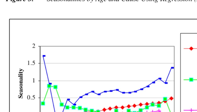
Figure 3: Seasonalities by Age and Cause Using Regression (Major Causes Only)
We can ask what causes of death contribute the most to the overall seasonality of deaths, in the period 1994 to 1998? To answer the question, for each age group i and cause j we calculated the seasonality of deaths in age group i excluding those who died of cause j. We then compared these to the seasonality of deaths for each age group i, obtaining the following:
0 0.5 1 1.5 2
0 10 20 30 40 50 60 70 80 90 100
Age
Seasonality
Cardiovascular
External Causes
Malignant Neoplasm
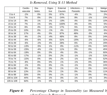
Table 4: Percentage Change in Seasonality in Each Age Group when Each Cause Is Removed, Using X-11 Method
Cardio-vascular
Dia-betes
Diges-tive
External Causes
Infections – Parasitic
Kidney Malignant Neoplasm
Respi-ratory
Other
0 to 4 -2% 0% 0% 67% -4% 2% 2% -24% 74%
5 to 9 7% 0% 0% -24% 9% -1% 23% 5% 37%
10 to 14 9% 1% 1% -19% 4% 0% 10% 5% 52%
15 to 19 7% 1% 0% -100% 4% 0% 5% 3% 27%
20 to 24 6% 4% -1% 17% 5% 0% 12% 1% 16%
25 to 29 10% 0% -1% 4% 25% 0% 6% 6% 4%
30 to 34 17% 4% 0% 87% 48% -3% -6% 3% 7%
35 to 39 4% -2% -4% 48% 8% 0% 24% -11% -19%
40 to 44 -6% -6% -6% 52% -20% -2% 32% -17% -4%
45 to 49 -6% -2% 3% 28% 6% -1% 29% -24% -4%
50 to 54 -13% -5% 1% 8% -11% 0% 34% -18% -3%
55 to 59 -23% -4% -1% 11% 0% 0% 45% -17% 0%
60 to 64 -19% 0% 0% 4% 0% -1% 60% -20% 0%
65 to 69 -17% -1% 0% 2% -1% -1% 53% -24% -4%
70 to 74 -22% 0% 0% 2% -1% 0% 52% -21% -4%
75 to 79 -8% 0% 0% 1% -1% 0% 36% -23% -1%
80 to 84 -1% 0% 0% 1% -1% 0% 24% -18% -3%
85 to 89 8% 0% 0% 1% -1% 0% 16% -18% -1%
90 to 94 13% 1% 0% 1% 0% 0% 11% -18% 3%
95 to 99 30% 0% 0% 1% -1% 0% 6% -17% -1%
100 to 104 44% 0% 1% 0% 1% -1% 3% -16% 10%
105 to 109 64% -1% 0% -2% -5% -1% -2% -19% 15%
Figure 4: Percentage Change in Seasonality (as Measured by the X-11 Method) when Cause Is Removed
-100% -50% 0% 50% 100%
0 10 20 30 40 50 60 70 80 90 100
Percentage
Cardiovascular
External Causes
Table 5: Percentage Change in Seasonality in Each Age Group when Each Cause Is Removed, Using Regression
Cardio-vascular
Dia-betes
Diges-tive
External Causes
Infections -Parasitic
Kidney Malignant Neoplasm
Respiratory Other
0 to 4 -3% -1% -2% 63% -10% 0% 2% -38% 127%
5 to 9 4% 0% -1% -33% 6% -1% 22% 5% 50%
10 to 14 11% 0% -1% -44% 9% 0% 17% 5% 35%
15 to 19 -5% 0% 0% -52% 4% -1% 6% 2% 18%
20 to 24 3% 1% -1% -14% 0% 0% 7% 2% 0%
25 to 29 -13% 2% 0% -100% 14% -1% 12% 3% -2%
30 to 34 N/A N/A N/A N/A N/A N/A N/A N/A N/A
35 to 39 N/A N/A N/A N/A N/A N/A N/A N/A N/A
40 to 44 -100% -7% -100% 114% 31% -3% 20% -100% -100%
45 to 49 -14% -4% 1% 28% 4% -2% 15% -20% -3%
50 to 54 -19% -4% 0% 10% -3% -1% 47% -19% -6%
55 to 59 -19% -4% 0% 6% -1% -1% 49% -19% -6%
60 to 64 -24% -2% -1% 5% -1% -1% 68% -20% -3%
65 to 69 -17% -2% -1% 2% -1% -1% 50% -21% -3%
70 to 74 -21% -1% 0% 1% -1% -1% 50% -20% -3%
75 to 79 -13% -1% 0% 1% -1% -1% 32% -18% -2%
80 to 84 -7% 0% 0% 1% -1% -1% 24% -16% -3%
85 to 89 2% 0% 0% 0% -1% -1% 15% -15% -2%
90 to 94 10% 0% 0% 0% 0% 0% 10% -16% -1%
95 to 99 23% -1% 0% 0% -1% 0% 5% -16% -1%
100 to 104 24% 0% 0% 0% 0% 0% 3% -13% 0%
105 to 109 19% 0% 0% 0% -1% -2% 1% -14% 7%
Figure 5: Percentage Change in Seasonality (as Measured by Regression) when Cause Is Removed
-150% -100% -50% 0% 50% 100% 150%
0 10 20 30 40 50 60 70 80 90
100
Age
Percen
tage
Cardiovascular
External Causes
Malignant Neoplasm
As we can see, cardiovascular and respiratory problems are the most significant factors for the seasonality of deaths in older people, while external causes are the most significant factors in younger people. Even though a large percentage of the population dies from malignant neoplasms, this cause depresses the overall seasonality of deaths in the whole population.
Seasonal patterns of mortality usually have winter excesses but not always: We found that younger people who die of external causes are more prone to die in the summer than in the winter. However, older people who die of external causes are more prone to die in the winter than in the summer.
3. Variation of Seasonality of Deaths with Respect to Age
The seasonality of death varied significantly among age groups, with a standard GHYLDWLRQRI DVODUJHDVWKHPHDQ IRUWKHQRQOLQHDUUHJUHVVLRQ PHWKRGDQGDVWDQGDUGGHYLDWLRQRI DVODUJHDVWKHPHDQ IRUWKH X-11 method. A natural question to ask is what is the reason for the large variation in the seasonalities of death with respect to age? Two possible factors are the variation in cause-seasonalities of death with respect to age and the variation in the distribution of causes of deaths with respect to age. We investigated how each of these factors affected the variation in age-seasonality.
To calculate the effect of the variation in cause-seasonalities of death with respect to age, we synthesized new functions,
∑
⋅ =j j ij i t n s t
s(1)() ()
where n is the number in age group i that died of cause j andij sj(t)is the overall
seasonality of deaths for people (in all age groups) that died of cause j. We define
seasonality of these new functions as we did before for sj(t). The following chart
displays boths and i (1)
i
Table 6: Degree of Seasonality of Deaths with and without Variation in Cause-Seasonality with Respect to Age
Age Group
i
s Computed Using
Nonlinear-Regression
) 1 (
i
s Computed Using
Nonlinear-Regression
i
s Computed Using the
X-11 Method
) 1 (
i
s Computed Using
the X-11 Method
0 to 4 0.05 0.22 0.08 0.25
5 to 9 0.34 0.08 0.39 0.11
10 to 14 0.32 0.07 0.34 0.09
15 to 19 0.22 0.07 0.22 0.08
20 to 24 0.16 0.07 0.16 0.07
25 to 29 0.11 0.06 0.12 0.08
30 to 34 0.00 0.08 0.07 0.12
35 to 39 0.00 0.10 0.07 0.14
40 to 44 0.04 0.12 0.08 0.15
45 to 49 0.08 0.14 0.09 0.17
50 to 54 0.10 0.15 0.13 0.18
55 to 59 0.13 0.16 0.14 0.19
60 to 64 0.15 0.18 0.17 0.21
65 to 69 0.16 0.19 0.20 0.23
70 to 74 0.19 0.21 0.22 0.24
75 to 79 0.23 0.23 0.27 0.27
80 to 84 0.28 0.24 0.33 0.29
85 to 89 0.33 0.26 0.39 0.31
90 to 94 0.36 0.27 0.42 0.32
95 to 99 0.40 0.28 0.50 0.33
100 to 104 0.43 0.29 0.48 0.34
105 to 109 0.54 0.30 0.63 0.36
The variance of (1)
i
s LV 2 = 0.0068 XVLQJ WKH QRQOLQHDU UHJUHVVLRQ PHWKRG DQG 2 =
0.0088 using the X-11 method. Then one minus the ratio of the standard deviation of )
1 (
i
s to the standard deviation of s is 45% for the non-linear regression method and 42%i
for the X-11 method. So we can estimate the percentage of the variation in seasonality attributable to the variation in the specific cause-seasonalities of death with respect to age as somewhere in the range of 42% to 45%.
And to calculate the effect of the variation in the distribution in causes of death with respect to age, we synthesized new functions,
∑
⋅ =j ij j i t n s t
s(2)() ()
where n is the total number of people that died of cause j andj sij(t)is the seasonality of
death in age group i that died of cause j. We define seasonality of these new functions
as we did before. The following chart displays boths and i (2)
i
s computed with each
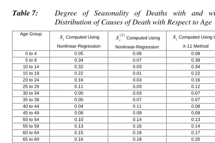
Table 7: Degree of Seasonality of Deaths with and without Variation in Distribution of Causes of Death with Respect to Age
Age Group
i
s Computed Using
Nonlinear-Regression
) 2 (
i
s Computed Using Nonlinear-Regression
i
s Computed Using the
X-11 Method
) 2 (
i
s Computed Using the X-11 Method
0 to 4 0.05 0.09 0.08 0.10
5 to 9 0.34 0.07 0.39 0.11
10 to 14 0.32 0.03 0.34 0.03
15 to 19 0.22 0.01 0.22 0.02
20 to 24 0.16 0.03 0.16 0.07
25 to 29 0.11 0.03 0.12 0.05
30 to 34 0.00 0.03 0.07 0.05
35 to 39 0.00 0.07 0.07 0.09
40 to 44 0.04 0.11 0.08 0.14
45 to 49 0.08 0.09 0.09 0.13
50 to 54 0.10 0.14 0.13 0.16
55 to 59 0.13 0.16 0.14 0.18
60 to 64 0.15 0.18 0.17 0.20
65 to 69 0.16 0.18 0.20 0.21
70 to 74 0.19 0.20 0.22 0.23
75 to 79 0.23 0.22 0.27 0.26
80 to 84 0.28 0.25 0.33 0.31
85 to 89 0.33 0.29 0.39 0.34
90 to 94 0.36 0.31 0.42 0.36
95 to 99 0.40 0.34 0.50 0.42
100 to 104 0.43 0.29 0.48 0.41
105 to 109 0.54 0.32 0.63 0.29
The variance of (2)
i
s LV 2 = 0.012 XVLQJ WKH QRQOLQHDU UHJUHVVLRQ PHWKRG DQG 2 =
0.0015 using the X-11 method. Then one minus the ratio of the standard deviation of )
2 (
i
s to the standard deviation of s is 27% for the non-linear regression method and 23%i
for the X-11 method. So we can estimate the percentage of the variation in seasonality attributable to the variation in the distribution of causes of death with respect to age as somewhere in the range of 23% to 27%.
Therefore, the variation in the seasonality of deaths with respect to age are substantially attributable to the variation in cause-seasonality with respect to age and to a lesser extent attributable to the variation in the distribution of causes of death with respect to age.
We present graphs of s ,i
) 1 (
i
s , and (2)
i
s computed using the X-11 method and
Figure 6: Seasonality of Deaths by Age in Real and Synthesized Cohorts Using the X-11 Method
Figure 7: Seasonality of Deaths by Age in Real and Synthesized Cohorts Using Regression
0.00 0.10 0.20 0.30 0.40 0.50 0.60 0.70
0 10 20 30 40 50 60 70 80 90
100
Age
S
eas
on
alit
y
Real
Synthesized 1
Synthesized 2
0.00 0.10 0.20 0.30 0.40 0.50 0.60
0 10 20 30 40 50 60 70 80 90 100
Age
S
eas
on
alit
y Real
Synthesized 1
4. Seasonality over the Years
We also used Social Security’s SSI records and the death file of the Office of the Chief Actuary (OCACT) at the Social Security Administration from 1976 to 1999. The OCACT death file is representative of the general population in the U.S. while the SSI death records only includes people who received supplemental security income (money from a needs based federal government program). Because the span of years in these files is so great, we did not use the non-linear regression method described earlier, since this method does not account very well for seasonality changing over time. (It only assumes a secular trend.) The following chart displays the average seasonality of deaths for each four-year period and each age group, using the X-11 method. We also calculated for each age group the correlation of single year of death with seasonality:
Table 8: Seasonality of Deaths from the SSI File by Years and Age Group with Correlation of Single Year of Death with Seasonality Using the X-11 Method
Age Group 1976-1979
1980-1983
1984-1987
1988-1991
1992-1995
1996-1999
Average Correlation
0 to 4 0.57 0.42 0.30 0.32 0.28 0.23 0.35 -0.90
5 to 9 0.27 0.39 0.40 0.38 0.37 0.45 0.38 0.70
10 to 14 0.41 0.24 0.27 0.32 0.29 0.21 0.29 -0.53
15 to 19 0.19 0.19 0.15 0.19 0.23 0.15 0.18 -0.04
20 to 24 0.18 0.13 0.10 0.12 0.10 0.11 0.12 -0.66
25 to 29 0.00 0.00 0.00 0.00 0.00 0.00 0.00 N/A
30 to 34 0.20 0.13 0.13 0.11 0.07 0.07 0.12 -0.91
35 to 39 0.13 0.10 0.10 0.07 0.06 0.07 0.09 -0.89
40 to 44 0.15 0.10 0.10 0.08 0.10 0.12 0.11 -0.38
45 to 49 0.17 0.12 0.08 0.11 0.09 0.11 0.11 -0.62
50 to 54 0.15 0.13 0.12 0.10 0.10 0.14 0.12 -0.33
55 to 59 0.18 0.15 0.12 0.12 0.12 0.17 0.14 -0.17
60 to 64 0.19 0.17 0.19 0.18 0.17 0.20 0.18 0.19
65 to 69 0.17 0.18 0.20 0.19 0.21 0.24 0.20 0.89
70 to 74 0.19 0.19 0.20 0.22 0.26 0.28 0.22 0.96
75 to 79 0.24 0.22 0.22 0.24 0.23 0.27 0.24 0.50
80 to 84 0.25 0.25 0.27 0.26 0.31 0.35 0.28 0.87
85 to 89 0.33 0.28 0.32 0.31 0.32 0.41 0.33 0.60
90 to 94 0.34 0.32 0.34 0.34 0.33 0.38 0.34 0.43
95 to 99 0.37 0.33 0.35 0.34 0.35 0.45 0.37 0.49
We did the same calculations for the death file of the Office of the Chief Actuary at the Social Security Administration (see Table 9).
Table 9: Seasonality of Deaths from the OCACT Death File by Years and Age Group with Correlation of Year of Death with Seasonality Using the X-11 Method
Age Group 1976-1979
1980-1983
1984-1987
1988-1991
1992-1995
1996-1999
Average Correlation
0 to 4 0.52 0.38 0.30 0.30 0.26 0.20 0.33 -0.92
5 to 9 0.31 0.30 0.31 0.34 0.31 0.30 0.31 0.13
10 to 14 0.45 0.34 0.24 0.22 0.24 0.15 0.27 -0.92
15 to 19 0.43 0.38 0.25 0.24 0.22 0.14 0.27 -0.94
20 to 24 0.30 0.31 0.18 0.13 0.15 0.12 0.20 -0.87
25 to 29 0.21 0.23 0.15 0.10 0.09 0.11 0.15 -0.85
30 to 34 0.11 0.12 0.10 0.09 0.07 0.06 0.09 -0.88
35 to 39 0.07 0.08 0.07 0.06 0.05 0.06 0.06 -0.62
40 to 44 0.09 0.09 0.09 0.06 0.07 0.07 0.08 -0.73
45 to 49 0.09 0.07 0.08 0.08 0.09 0.11 0.09 0.71
50 to 54 0.14 0.11 0.11 0.09 0.10 0.12 0.11 -0.55
55 to 59 0.15 0.11 0.11 0.11 0.12 0.15 0.13 0.03
60 to 64 0.17 0.14 0.13 0.15 0.16 0.17 0.15 0.34
65 to 69 0.16 0.15 0.16 0.16 0.17 0.19 0.16 0.76
70 to 74 0.18 0.18 0.18 0.18 0.20 0.22 0.19 0.81
75 to 79 0.21 0.19 0.20 0.22 0.24 0.28 0.22 0.84
80 to 84 0.25 0.25 0.25 0.25 0.29 0.33 0.27 0.84
85 to 89 0.28 0.26 0.31 0.32 0.35 0.38 0.32 0.92
90 to 94 0.34 0.31 0.33 0.35 0.38 0.42 0.36 0.81
95 to 99 0.41 0.38 0.39 0.39 0.45 0.49 0.42 0.73
100 to 104 0.41 0.45 0.46 0.45 0.46 0.48 0.45 0.78
105 to 109 0.70 0.62 0.48 0.61 0.62 0.61 0.61 -0.23
Figure 8: Average Seasonality of Deaths by Age
Figure 9: Correlation of Seasonality with Year of Death
-1,00 -0,80 -0,60 -0,40 -0,20 0,00 0,20 0,40 0,60 0,80 1,00
0 10 20 30 40 50 60 70 80
90 100
Age
Correlat
ion
OCACT Death File
SSI Death File 0,00
0,10 0,20 0,30 0,40 0,50 0,60 0,70 0,80
0 10 20 30 40 50 60 70 80
90 100 Age
Seas
onalit
y OCACT Death File
As we observed before, seasonality is greater for the more vulnerable cohorts, the young and the old. We also see that in general, seasonality of deaths decreased over time for the younger age groups and increased over time for the older age groups. Even though the people in the SSI population are generally poorer than those in the general population, the seasonalities of death are similar in each group; therefore, we have evidence that the seasonality of death phenomenon is not strongly influenced by economic status.
We now summarize our main findings:
• The X-11 variation of Census Method II and non-linear regression methods give
similar measures of seasonality (for each subgroup of the population).
• The most vulnerable subgroups of the population (the young and the old) have
the most seasonal variation in death.
• Respiratory and cardiovascular causes of death contribute the most to the overall
seasonal excesses in the winter (for the old), while external causes of death contribute the most to the overall seasonal excesses in the summer (for the young).
• The large variation in seasonality with respect to age is attributable substantially
to the variation in cause-seasonality with respect to age (42% to 45%). It is also somewhat attributable to the variation in the distributions of causes with respect to age (23% to 27%).
• The seasonalities of deaths have been increasing over the years (from 1976 to
1999) for older people and decreasing for younger people.
• There is evidence that seasonality of deaths is not heavily influenced by
economic status.
5. Acknowledgements
I would like to thank Bert Kestenbaum for his thorough review of this paper and his many suggestions, including the idea that I investigate the topic of seasonality of mortality. Also, I thank the Max Planck Institute for Demographic Research for sponsoring and inviting me to the seminar at Duke University which was very helpful for learning about research done on seasonality of mortality in different countries. And I would like to thank Reneé Ferguson for suggesting to me the method that I used which measured the statistical significance of the added parameters in the nonlinear regression procedure. Last but not least, I would like to thank Michael Stephens for helping me
References
Gemmell I., McLoone P., Boddy F.A., Dickinson G.J., Watt G.C.M., 2000, “Seasonal Variation in Mortality In Scotland”, International Journal of Epidemiology, 29: 274-279.
Kalkstein, L. S., Valimont K. M., 1987, Climate effects on human health. In Potential
effects of future climate changes on forests and vegetation, agriculture, water resources, and human health. EPA Science and Advisory Committee
Monograph no. 25389, 122-52.
Laake K., Sverre J.M., 1996, “Winter Excess Mortality: A Comparison Between Norway and England Plus Wales”, Age and Aging, 25:343-348.
Mackenbach J. P., Kunst A. E., Looman C. W. N., 1992, “Seasonal Variation in Mortality in The Netherlands”, Journal of Epidemiology and Community Health, 46: 261-265.
Rogot E., Fabsitz R., Feinleib M., 1976, “Daily Variation in USA Mortality”, American
Journal of Epidemiology, Vol. 103 No. 2: 198-211.
Rogot E., Padgett S.J., 1976, “Associations of Coronary and Stroke Mortality With Temperature and Snowfall In Selected Areas of the United States”, American
Journal of Epidemiology, Vol. 103 No. 6: 565-575.
Rosenwaike I., 1966, “Seasonal Variation of Deaths in the United States, 1951-1960”,
Journal of the Amercian Statistical Association, Vol. 61: 706-717.
Seretakis D., Lagiou P., Lipworth L., Signorello LB., Rothman KJ., Trichopoulos D., 1997, “Changing Seasonality of Mortality From Coronary Heart Disease”,
JAMA, 278(12):1012-4.