AUT J. Model. Simul., 49(2)(2017)217-226 DOI: 10.22060/miscj.2017.11945.4985
3-RPS Parallel Manipulator Dynamical Modelling and Control Based on SMC
and FL Methods
M. Shahidi1*, J. Keighobadi1, A. R. Khoogar2
1 Faculty of Mechanical Engineering, University of Tabriz, Tabriz, Iran
2 Department of Mechanical Engineering, Maleke-Ashtar University of Technology, Tehran, Iran
ABSTRACT: In this paper, a dynamical model-based SMC (Sliding Mode Control) is proposed for trajectory tracking of a 3-RPS (Revolute, Prismatic, Spherical) parallel manipulator. With ignoring small inertial effects of all legs and joints compared with those of the end-effector of 3-RPS, the dynamical model of the manipulator is developed based on Lagrange method. By removing the unknown Lagrange multipliers, the distribution matrix of control input vector disappears from the dynamical equations. Therefore, the calculation of the aforementioned matrix is not required for modeling the manipulator. It in trun results in decreased mathematical manipulation and low computational burden. As a robust nonlinear control technique, a SMC system is designed for the tracking of the 3-RPS manipulator. According to Lyapunov’s direct method, the asymptotic stability and the convergence of 3-RPS manipulator to the desired reference trajectories are proved. Based on computer simulations, the robust performance of the proposed SMC system is evaluated with respect to FL (feedback linearization) method. The proposed model and control algorithms can be extended to different kinds of holonomic and non-holonomic constrained parallel manipulators.
Review History:
Received: 5 September 2016 Revised: 26 February 2017 Accepted: 9 May 2017 Available Online: 21 June 2017 Keywords:
Parallel manipulator Dynamic modeling Trajectory tracking Feedback linearization sliding mode control 1- Introduction
In recent decades, parallel manipulators have been widely studied because of their satisfactory performance criteria such as rigidity, accuracy and high weight/load ratio. These kinds of manipulators are widely used in practical applications, including flight vehicle simulators, high-precision machining centers, assembly lines, and pick and place robotic arms and are becoming increasingly popular in the industry. On the other hand, the main drawbacks of these manipulators are small workspace and difficult mathematical modeling. Generally speaking, forward kinematic modeling of parallel robots is regarded as a challenge. In spite of developing analytical direct kinematic models of some special structures [1-3], the generalized coordinates of the end-effector cannot be usually expressed as analytical terms of actuated joints coordinates . Since the solution of the forward kinematic is not unique, some techniques have been presented to find all the possible solutions of the forward kinematic problem. It should be noted that there exists no algorithm that addresses the current pose of the platform among the set of solutions. Numerical methods using a-priori information on the current pose are also developed. These methods are more compatible with a real-time approach [4]. One of the most popular methods is the Newton’s method which is used in this paper. If the initial approximation for the coordinates of the moving platform is sufficiently close to its real coordinates, this method yields the exact solution [5, 6].
By the same token, the dynamical model of parallel manipulators which is particularly required to build up a control system has a tendency to be very complicated due to kinematic constraints and closed-loop structure [7]. Most
studies on the dynamics of these manipulators are based on the Newton–Euler method, the Lagrangian formulation, and the principle of virtual work. The aforementioned dynamical equations are accurate by containing actuating legs having connections to each other in their formulation. The computation of the dynamics is very time-consuming [8]. In [9], developing forward dynamical model for the six limbs Stewart platform based on Kane’s equation is proposed. Khalil and Guegan [10] presented closed-form solutions for the complete inverse and forward dynamical models of the Stewart manipulator robot. The models are established in terms of the dynamical models of the legs. For modeling a 3-RPS parallel manipulator using Lagrange method, Pendar et al. [11] introduces a formulation scheme in which the natural orthogonal complement matrix for omitting Lagrange multipliers can be found by the inverse calculation of some of 2×2 matrices instead 9×9 ones. A linear modeling method for parallel robots based on observable kinematic elements is proposed in [12]. In [13], by implementing an approach that deals with a reduced dynamical model with a physically feasible set of parameters, a simplified model based on a set of relevant parameters is developed. There, it is shown that the controller design for the reduced model leads to a better trajectory tracking compared with the control system developed based on the complete set of dynamic parameters. The problem of controlling robotic manipulators has earned the interest of many authors during the present decade. Like many engineering applications, in robotics, it is impossible or rather challenging to attain an exact dynamical model of a robot, due to the existence of flexibility, backlash, Coulomb friction, a variation of payload, unidentified disturbances, the coupling of limbs, and time-varying parameters [14, 15]. Therefore, the mathematical model of a robot is always an approximation of the real robot. Accordingly, control
schemes considered for controlling a robot should be robust, fast convergent and have a simple structure. Sirouspour and Salcudean [16] focus on the control problem of hydraulic robot manipulators where a controller is further improved with adaptation laws to compensate for parameter uncertainties in the system dynamics. In the research work by Davliakos and Papadopoulos [17] a model-based controller is developed for an electro-hydraulic Stewart manipulator in which rigid body equations of motion and hydraulics dynamics, including friction and servo valve models, are considered. Khosravi and Taghirad study PID control of fully-constrained cable-driven parallel robots in the presence of structured and unstructured uncertainties in the dynamics of the robot [18]. As a approach to the robust control, sliding mode control is receiving attention. The advantages of using sliding mode control are its fast response, good transient performance and robustness against disturbances and noises [14, 19-21].
In the current paper, following the inverse and forward kinematical modeling, under the assumption that the leg inertia is negligible, the dynamical model of the 3-RPS manipulator is obtained using Lagrange method. Considering six dependent generalized coordinates in the modeling process, and by applying the principle of virtual work, the distribution matrix of control input vector in the formulation appears as an identity matrix. Therefore, mathematical manipulation and computational burden significantly decrease. The present method can be applied to nonholonomic systems as well. With following linearization, the error dynamics of the 3-RPS through the computed torque method, an SMC law is applied to stabilize the robot around its reference trajectories even in the presence of exogenous disturbances, and uncertainties in the model . Through software simulation, the superiority of the proposed control system is compared with a FL control method. As can be seen, both the SMC and FL control systems yield the convergence of the end-effector to the reference trajectory when there is no disturbance and no parameter uncertainty. Although disturbances do not affect the performance of the FL controller, parameter uncertainties especially uncertain geometrical specifications lead to malfunction of the FL controller. However, as a robust control approach, the proposed SMC system results in satisfactory tracking performance against all the above-mentioned uncertainties and exogenous inputs.
The rest of the paper is organized as follows. In section 2 kinematic and dynamic models of the 3-RPS is obtained. The the control system design is explained in section 3. In section 4, to assess the significance of the proposed SMC system, the tracking of sinusoidal paths is simulated. Concluding remarks and analyses are presented in section 5.
2- Modelling of the manipulator 2- 1- Kinematic Modelling
To develop the kinematical model of the 3-RPS parallel manipulator, at first, the closed form solution of inverse kinematics is represented for displacement, velocity, and acceleration based on the method proposed in [4] and [22]. With the use of the inverse kinematical model, the linear displacement, velocity, and acceleration of the three links are given in terms of three dimensional position and Euler angles of the end-effector.
The most classical way for describing the pose of a moving
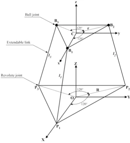
platform is to use the coordinates of a reference frame at a given point C in the body and three or more parameters to express its orientation. In this research work, by considering the workspace of the manipulator, a set of Euler angles (j,q,y) which uniquely determines the orientation of a rigid body by the sequence of rotations x-y-z (or 1-2-3) is used. The kinematic sketch of the 3-RPS manipulator and coordinate systems used for describing position and orientation of the moving platform are depicted in Figures 1 and 2, respectively.
Fig. 1. Schematics of the structure for a typical 3-RPS
The frame XYZ is a fixed coordinate system located at the center of the base platform in which Z-axis is vertically upward and the X-axis is pointing toward the revolute joint P1. The frame X’Y’Z’ is a nonrotating coordinate system that translates with the end-effector and its axes are parallel to the axes of XYZ frame. The frame xyz is a body coordinate system that rotates with the end-effector. It is attached to the center of the end-effector, with the z-axis normal to the moving platform and the x-axis pointing towards the ball joint B1. The end-effector is connected to the limbs by means of ball joints.
As shown in Figure 2, it is considered that both ball and revolute joints are placed at vertices of the two equilateral triangles which are laid at the moving and base platform, respectively. The ball joints are set at radius r from the moving platform center while the revolute joints are connected to the base platform radius R from the center of the base platform. As the link length varies, the end-effector is manipulated with respect to the base platform.
The transformation from the body to the fixed coordinate frame is described by the following equation [23]:
Before proceeding to the inverse kinematic modeling, it is useful to express the angular velocity w=(wxwywz)T and the angular acceleration a=(ax ay az)T of the moving platform with respect to frame XYZ as functions of the first and the second-time derivatives of the Euler angles.
Refer to Figure 2. the coordinates of the i-th joint on the moving platform, with respect to the fixed coordinate system XYZ is attained using the following equation.
In equation (4), bi is the coordinates of the i-th spherical joint Bi on the moving platform, described with respect to xyz
frame and C=(Xc Yc Zc)T is the position vector of the moving platform center (origin of the xyz frame) with respect to the XYZ coordinate system. Once the position of the attachment Bi is determined, the vector Li is simply computed as:
where Pi is the position vector of the i-th revolute joint defined in XYZ coordinate system. The length and the direction of the i-th link can be simply computed from the following equations:
It should be noted that the links l1, l2 and l3 are constrained by the revolute joints. Therefore, according to the chosen structure of the manipulator, the ball joints B1, B2 and B3 are constrained to move in the planes Y=0, Y=−√3X, and Y=√3X respectively.
Inserting these constraints in equation (4) leads to the following constraint equations:
where tij is the entry of transformation matrix T that is placed in the i-th row and j-th column. Considering the constraints equations, it can be seen that the manipulator has two orientational degrees of freedom and one degree of translation freedom.
In order to solve the inverse rate kinematics problem, the velocity of point Bi should be obtained first. This can be accomplished by calculating time derivative of equation (4) which leads to the following equation.
The i-th link extension rate is the projection of this velocity vector along the direction vector of the link. Thus, the links extension rate can be calculated using equation (12).
The above equation represents the solution to the inverse rate kinematics problem. Considering the fact that for a triple scalar product a×b.c the dot and cross products can be changed yielding a.b×c, equation (12) can be rewritten by: (1) (5) (6) (7) (2) (8) (9) (10) (11) (12) (13) (3) (4)
=
−
i i i
L
B
P
= +
i i
B C
Tb
.
=
i i il
L L
[
]
ˆ
=
T=
ii iX iZ iZ
i
L
n
n
n
n
l
11 22 ( ) 2 = − C rX t t
21
= −
CY
rt
1 12 21
tan
−
=
⇒ =
−
+
S S
t
t
C
C
j q
y
j
q
= + ×
i iB
C
w
Tb
ˆ
ˆ
ˆ
.
.
.
=
=
+ ×
i
i i
i i il
B n C n
w
Tb n
1 2 3 3 6×
=
l l lT W Xc Yc Zc j q y T
′ ′ = ′ − = + − − − +
X x Y y Z zC C C S S
C S S S C C C S S S S C
S S C S C S C C S S C C
T
T
q y q y q
j y j q y j y j q y j q
j y j q y j y j q y j q
1 0 0 0 = = − = X Y Z S
C S C E
S C C
w
q
j
j
w
w
j
j q q
q
w
j
j q y
y
=
=
+ −
−
+
−
−
X Y ZE
C
S
C C
S S
C
S C
C S
a
j
a
a
q
a
y
qy q
where:
The matrix W constitutes the first three rows of the Jacobian matrix. To achieve a 6×6 full inverse kinematic jacobian matrix, the other rows are obtained from time derivatives of the constraint equations (8), (9) and (10). This leads to the following inverse Jacobian matrix:
The acceleration of point Bi can be calculated by differentiating equation (11) with respect to time.
Now, can be simply obtained from the time-derivative equation (12).
By rewriting equation (5) in the form , is computed as:
The forward kinematic problem is indeed more complicated for parallel manipulators. It is equivalent to solve the nonlinear system of inverse kinematics equations and there exists usually more than one solution. For a given set of link lengths, the number of solutions corresponds to the number of configurations into which the mechanism can be
assembled. [4, 24].
A standard method to solve a non-linear system of equations is the Newton iterative scheme. Considering the generalized coordinate vector of the moving platform, q is a function of the known joint variables vector as:
and that q0 is the initial estimate for the solution of the forward kinematic problem, the iterative Newton formulation at iteration k is:
The iterating stops when where e is a
constant threshold. It can be shown that the matrix
is the same as the inverse Jacobian matrix J-1 given by equation (16) [25].
2- 2- Dynamical model
In order to accurately control a manipulator, a dynamic model is essential. As it follows, the relations between the generalized accelerations, velocities, coordinates of the end-effector and the joint forces are determined using Lagrange method. Although the 3-RPS manipulator has three holonomic constraints, a method is adopted which can also be used for nonholonomic systems. With ignoring small inertial effects of all legs and joints compared with that of the end-effector of 3-RPS, generalized coordinates and Lagrangian are considered as:
With applying the Lagrange method, the following equation is obtained:
And the kinematic constraints are written in the form:
where M(q)∈R6×6 is a positive definite matrix;
is the term which may include centripetal and Coriolis forces; D(q) is a 6×3 full rank distribution matrix of input control vector; A(q) is a 3×6 full rank matrix associated with the constraints. F=[F1 F2 F3]T is the control input vector and l∈R3 is the constraint force vector. Let Ni = Ni(q), i = 1,2,3 be a set of smooth and linearly independent functions such that :
and D be the distribution spanned by the vectors Ni, then from
(
)
(
)
(
)
1 1 1
3 3 3 3
2 2 2
3 3 3 3 3 ˆ 0 ˆ 0 ˆ × × × × = × × T T T T T T
n Tb n I
W n Tb n
E Tb n n (14) (15) (19) (20) (16) (21) (22) (23) (24) (25) (17) (18)
(
)
(
)
(
)
1611 12 13 14 15
26
21 22 23 24 25
36
31 32 33 34 35
1 1 1 1 46 44 45 1 1 56 55 1 66 1 44 1 45 1 46 1 55 1 56
2 0
0
0
1
0
0
0
0
0
(
)
− − − − − − − − − − − −
=
−
=
+
=
−
=
+
−
=
= −
w
w
w
w
w
w
w
w
w
w
w
w
w
w
w
w
w
w
J
J
J
J
J
J
J
S
S
J
r C S S
S C
J
r S C S
S C
J
r S S C
S C
C
J
rS S
J
q
j
j q y
j y
j q y
q y
j q y
y j
q
q y
(
)
2 2 21
66
1
−
=
+
+
+
rC C
C
C
S S
J
C C
q y
j
q
j q
j q
(
)
= + ×
+ ×
×
i i iB
C
a
Tb
w w
Tb
il
ˆ
ˆ
.
.
=
+
i
i i
i il
B n
B n
ˆ
=
+
i i i i
B
P l n
n
ˆ
iˆ
ˆ
=
−
i i ii
i
B
l n
n
l
( )
=
l G q
( )
1(
( )
)
1
0,1,...
− +∂
=
−
−
∂
=
kk k k given
G q
q
q
G q
l
q
k
( )
k−
given≤
G q
l
e
( )
∂ ∂ k G q q[
]
=
c c c Tq
X
Y
Z
j q y
(
2 2 2) (
2 2 2)
1 1
2 2
= p c + c + c + xx x + yy y + zz z
L m X Y Z I w I w I w
( )
+
( )
,
=
( )
+
T( )
M q q V q q
D q F A q
l
6 ( , ) ∈
V q q R
( )
i=
0,
=
1, 2,3
A q N
i
( )
=
0
A q q
[
1 2 3]
= T
(24) it follows that , that is, there exists a 3-dimensional pseudo-velocity vector S=[S1 S2 S3]T such that:
where N6×3=[N1(q) N2(q) N3(q)]. In order to satisfy equations (25) and (26), S and N are chosen as:
Differentiating from (26), we obtain:
Substituting (29) in (23) and premultiplying by NT, we have:
It should be noted that there is no need to premultiply (30) by (NTD)-1. Because NTD will be a 3×3 identity matrix and automatically disappears from the equation. The aforementioned statement can be proven by applying the principle of virtual work [26] for the 3-RPS manipulator.
where t∈R6 is the generalized forces vector and d represents the virtual displacement. Regarding equation (13), we can write:
With substituting (32) in (31) leads to:
Since in equation (23), D(q)F represents the generalized forces, it can be concluded that:
Thus NTD is calculated as:
This fact considerably lowers mathematical manipulation of Lagrange method applied to the constrained parallel manipulators. The distribution matrix of input control vector D(q) disappears from the dynamical equations and the inversion of NTD is not required. Now the mechanical systems (23) can be reduced to the following form:
where is a 3×3 matrix and
is a 3×1 matrix.
The represented method for mathematically modeling of the 3-RPS could be extended to different kinds of constrained parallel manipulators.
3- Controller design 3- 1- Problem statement
The purpose of SMC design is to generate the control inputs, F=[F1 F2 F3]T which makes the 3-RPS track a feasible desired trajectory. The six-dimensional posture variables of reference trajectory are defined as qr=[Xcr Ycr Zcrjrqryr]T. The reference velocity and acceleration vectors are
and respectively, which are obtained from qr and its time derivatives. In the reference trajectory qr, the dependent components are computed based on the constraint equations (8) to (10).
Considering inherent perturbations like parameter uncertainties, disturbances, and nonlinearities, we have:
where Fp=[F1p F2p F3p]T is defined as perturbation to the dynamic equation (36). It is assumed that Fp is bounded and is a multiplier of matrix , i.e. satisfies the uncertainty matching condition.
f1m, f2m and fm are upper bounds of perturbations.
3- 2- Controller design
Let the position and orientation errors be
To satisfy the tracking requirements, sliding surfaces are defined by:
where g1, g2, and g3 are positive constants. If the sliding surfaces are stabilized, the convergence of the 3-RPS manipulator to the reference trajectory is guaranteed. Control inputs are defined by the computed-torque method as a feedback-linearization method [27] as:
(26)
(27)
(28)
(29)
(30)
(31)
(37)
(38)
(39)
(40)
(41)
(42) (32)
(33)
(34)
(35)
(36)
∈ D
q
=
q NS
1 2 3
=
T
S
l l
l
11 21 31 41 51 61
12 22 32 42 52 62
13 23 33 43 53 63
=
T
J
J
J
J
J
J
N
J
J
J
J
J
J
J
J
J
J
J
J
=
+
q NS NS
+
+
=
T T T T
N MNS N MNS N V
N DF
=
T T
l F
q
d
d t
=
T T T
l
q W
d
d
=
TW F
t
=
TD W
1 0 0
0 1 0
0 0 1
=
=
T T T
N D N W
( , )
=
+
=
q NS
MS V q S
F
=
T
M N MN V N MNS N V= T + T
1 2 3
= T
r r r r
S l l l
1 2 3
=
T
r r r r
S l l l
(
,
)
+
+
=
pMS V q S
F
F
M
= ×
p
F M f
[
1 2 3]
1 1
,
2 2,
3 3=
≤
≤
≤
T
m m m
f
f
f
f
f
f
f
f
f
f
= −
= −
=
−
e r
e r
ce c cr
Z
Z
Z
j
j j
q
q q
1 1
2 2
3 3
=
+
=
+
=
+
e e
e e
ce ce
s
s
s
Z
Z
j g j
q
g q
g
(
, ,
)
=
r+
+
where U=[u1 u2 u3]T is the control law. Applying control input (42) in the dynamic equation of the 3-RPS (36), we have the feedback-linearized dynamic equation as:
In what follows, the control laws u1, u2 and u3 which stabilize the sliding surfaces s1, s2 and s3 are proposed.
where hi, gi, bi, and ei are real positive constant values for i=1,2,3 and bi > hi , ei > fim .
To prove the stability of s1, s2 and s3 when u1, u2 and u3 are applied, Lyapunov direct method is used. With inserting u1 , u2 and u3 in (41), are derived as:
According to the Lyapunov direct method, we introduce the following Lyapunov function:
The time derivative of V along the trajectory is given by:
From (45), (46), (47), and (49), one attains
Therefore, s1, s2, and s3 are asymptotically stable and the 3-RPS manipulator converges to the reference trajectory. The block diagram of the proposed control system is shown
in Figure 3. It should be noted that using sign function in controller design when posture errors are negligible causes chattering. To weaken this phenomenon, we can use some continuous functions to approximate sign function. For instance, saturation or sigmoid function can be used instead.
4- Simulation results
To verify the effectiveness of the proposed SMC, a software simulation is run for tracking the sinusoidal trajectories of desired position and orientation of the end-effector. The performance of the proposed SMC system is compared with the classic FL control method under large initial off-tracks. According to Figures 4 through 6, when using both the FL and SMC systems, the end-effector of the 3-RPS converges to the corresponding desired values. As an important performance index, the actuator forces of both the FL and SMC systems are shown in Figures 7 to 9. In the reaching phase to the desired trajectories, in spite of a large upper bound on actuator forces, the reaching time obtained from the FL control system is larger than that the SMC yields. Consequently, the superior performance of the proposed SMC is concluded.
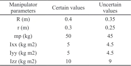
In order to investigate the robustness of the proposed control systems against disturbances and parameter uncertainties, two kinds of disturbance vectors are considered in simulations. The first disturbance is a step of magnitude 100 N; and the second is a 1 Hz sinusoidal disturbance of amplitude 100 N. Finally, with considering uncertainty on the geometrical and inertial parameters of the manipulator as in Table 1, the performance of the control methods is investigated.
The tracking errors of the angles j and q and the displacement along axis Z in the presence of the step disturbance are depicted in Figures 10 through 12. The steady state tracking errors along the desired trajectories of angles j and q by the FL method are smaller than those achieved from the SMC system. However, unlike the SMC, there is a remarkable steady-state error in the tracked path along the Z axis. Through imposing the sinusoidal disturbance, the above-explained tracking errors are denoted in Figures 13 to 15. In this case, the SMC shows an accurate performance when compared to the FL system in the tracking of all independent coordinates, j, q and Zc.
The main advantage of the SMC method appears when there exist geometrical and inertial uncertainties. As can be seen in Figures 16 and 17, the parameter uncertainties, especially
+ =
+
rS f
S U
(43)(44)
(45)
(46)
(47)
(48)
(49)
(50)
1 1 1 1 1 1 1
1 1
2 2 2 2 2 2 2
2 2
3 3 3 3 3
3 3 3 3
sgn(
)
sgn( )
sgn(
)
sgn( )
sgn(
)
sgn( )
= −
−
−
−
−
−
= −
−
−
− −
−
= −
−
−
−
−
−
r e e e e e
r e e e e e
r ce ce ce
ce ce
u
l l
s
s
u
l
l
s
s
u
l l
Z
Z
Z
Z
s Z
s
h j g j j
b j
j
e
h q g q q
b q
q
e
h
g
b
e
,
e eand Z
cej q
1 1 1 1
1 1 1
sgn(
)
sgn( )
= −
−
−
−
−
e e
e es
es
f
j
h j g j
b j
j
e
1 2 2 2
2 2 2
sgn(
)
sgn( )
= −
−
−
−
−
e e
e es
es
f
q
h q g q b q
q
e
3 3 3 3
3 3 3
sgn(
)
sgn( )
= −
−
−
−
−
ce ce
ce ce ceZ
Z
Z
Z
s Z
s
f
h
g
b
e
2 2 2
1 2 3
1 (
)
2
=
+
+
V
s
s
s
(
)
(
1 1 2 2)
3 3(
1)
12 2 3 3
=
+
+
=
+
+
+
+
+
e e
e e ce ce
V
s s s s
s s
s
s
s Z
Z
j g j
q
g q
g
1 1 1 1 1 1 1 1
2 2 2 2 2 2 2 2
3 3 3 3 3 3 3 3
= −
−
−
−
−
−
−
−
−
−
−
−
e ee e
ce ce
V
s
s
s
f s
s
s
s
f s
s Z
Z s
s
f s
b j
h j e
b
q
h q
e
b
h
e
Fig. 3. Block diagram of proposed SMC system
TABLE 1. Strouhal number for different geometric cases Manipulator
parameters Certain values Uncertain values
R (m) 0.4 0.35
r (m) 0.3 0.25
mp (kg) 50 45
Ixx (kg m2) 5 4.5
Iyy (kg m2) 5 4.5
Fig. 4. Tracking performance of angle, j
Fig. 7. Produced force by the first prismatic joint
Fig. 8. Produced force by the second prismatic joint
Fig. 9. Produced force by the third prismatic joint Fig. 5. Tracking performance of angle, q
Fig. 6. Tracking performance along Z axis Fig. 10. Tracking error of angle, j under step disturbance
geometrical ones lead to the weak performance of the FL controller unlike the superior performance of the SMC system. Since the geometrical uncertainties in Table 1 do not significantly affect the performance of the manipulator along the Z axis, the corresponding tracking error is short by the FL control system, see Figure 18.
5- Conclusion
This paper outlined mathematical modeling and control problem of a 3-RPS parallel robot. Although the 3-RPS has three holonomic constraints, six dependent generalized coordinates were used for dynamical modeling. It was shown that by choosing links extension rates as the components of a pseudo-velocity vector, and the first three columns of Jacobian matrix as a natural orthogonal complement, removing unknown Lagrange multipliers leads to a reduced Fig. 13. Tracking error of angle, j under sinusoidal disturbance
Fig. 16. Tracking error of angle, j in the presence of parameter uncertainties
Fig. 14. Tracking error of angle, q under sinusoidal disturbance
Fig. 17. Tracking error of angle, q in the presence of parameter uncertainties
Fig. 12. Tracking error along Z axis under step disturbance
Fig. 15. Tracking error along Z axis under sinusoidal disturbance
dynamical model in which the distribution matrix of control input vector is identity. While Lagrange method is widely used in the modeling of parallel robots, this paper proposed a new and straightforward modeling algorithm for modeling constrained parallel manipulators. As a robust nonlinear control approach, the SMC system was used for the trajectory tracking of the manipulator. Using Lyapunov direct method, the asymptotic stability of the proposed control system is proved. Simulations with the typical desired trajectory inputs were presented, and the results were compared with an FL control system. It was shown the proposed SMC system leads to a faster compensation of the initial off-tracks while the produced force by the prismatic joints is lower than that of the FL. Given uncertainties in both inertial and geometrical parameters of the manipulator, through simulation under step and sinusoidal disturbances, the satisfactory performance of the SMC controller was investigated.
Appendix A.
The detailed expressions of the matrices M(q) and A(q) and vector are given by:
Where:
References
[1] P. Nanua, K.J. Waldron, V. Murthy, Direct kinematic solution of a Stewart platform, IEEE Transactions on Robotics and Automation, 6(4) (1990) 438-444.
[2] P. Ji, H. Wu, A closed-form forward kinematics solution for the 6-6/sup p/Stewart platform, IEEE Transactions on robotics and automation, 17(4) (2001) 522-526.
[3] J. Schadlbauer, D. Walter, M. Husty, The 3-RPS parallel manipulator from an algebraic viewpoint, Mechanism and Machine Theory, 75 (2014) 161-176.
[4] J.-P. Merlet, Parallel robots, Springer Science & Business Media, 2006.
[5] J.-P. Merlet, Direct kinematics of parallel manipulators, IEEE transactions on robotics and automation, 9(6) (1993) 842-846.
[6] C.-f. Yang, S.-t. Zheng, J. Jin, S.-b. Zhu, J.-w. Han, Forward kinematics analysis of parallel manipulator using modified global Newton-Raphson method, Journal of Central South University of Technology, 17(6) (2010) 1264-1270.
[7] W.-H. Ding, H. Deng, Q.-M. Li, Y.-M. Xia, Control-orientated dynamic modeling of forging manipulators with multi-closed kinematic chains, Robotics and Computer-Integrated Manufacturing, 30(5) (2014) 421-431.
[8] S.-H. Lee, J.-B. Song, W.-C. Choi, D. Hong, Position control of a Stewart platform using inverse dynamics control with approximate dynamics, Mechatronics, 13(6) (2003) 605-619.
[9] M.-J. Liu, C.-X. Li, C.-N. Li, Dynamics analysis of the Gough-Stewart platform manipulator, IEEE Transactions on Robotics and Automation, 16(1) (2000) 94-98.
[10] W. Khalil, S. Guegan, Inverse and direct dynamic modeling of Gough-Stewart robots, IEEE Transactions on Robotics, 20(4) (2004) 754-761.
[11] H. Pendar, M. Vakil, H. Zohoor, Efficient dynamic equations of 3-RPS parallel mechanism through Lagrange method, in: Robotics, Automation and Mechatronics, 2004 IEEE Conference on, IEEE, 2004, pp. 1152-1157.
[12] E. Özgür, N. Andreff, P. Martinet, Linear dynamic modeling of parallel kinematic manipulators from observable kinematic elements, Mechanism and Machine V(q,q)
( )
44 45
54 55
0 0 0
0 0
0 0 0
0 0
0 0
0 0 0
0 0 0
0
0 0 0
0 0 0 0
= p p p zz zz zz m m m M q
M M I S
M M
I S I
q
q
(A.1) (A.2) (A.3) (A.4) (A.5) (A.6) (A.7) (A.8) (A.9)( )
1 1 1
44 45 46
1 1
55 55
1 66
2 0 0
0 1 0 0
0 0 0
− − − − − −
−
=
J
J
J
A q
J
J
S
q
S
j
J
( )
,
=
0 0
4 5 6
T p
V q q
m g V V V
(
)
2(
)
2( )
244
=
xx+
yy+
zzM
I C C
q y
I C S
q y
I S
q
(
)
(
)
45
=
54=
xx−
yyM
M
I
I
C S C
q y y
( )
2(
)
255
=
xx+
yyM
I
S
y
I C
y
(
)
(
)
(
)
(
)
(
)
(
)
4 [ ] [ ] = − − + − + + − − − + − + + xx x yy y zz zV I C C S C C S C
S C C S
I C S S S C C S
S S C C
I S C C
q y jq q y jy q y qy y w q q y y q y
q y jq q y jy q y qy y w q q y y q y
jq q q w q q
(
)
(
)
(
)
(
)
(
)
5[
]
[
]
=
−
−
+
+
+
−
−
−
+
−
xx x yy y zz zV
I S
C
S C
C S
S C
C
I C
S S
C C
S
S C
S
I
C
y qy y jq q y jy q y
w j q y y y
y jq q y jy q y qy y
w j q y y y
w j q
(
)
(
)
6
=
−
+
+
+
xx x yy y zzV
I
C S
C
I
C C
S
I
C
Theory, 69 (2013) 73-89.
[13] M. Diaz-Rodriguez, A. Valera, V. Mata, M. Valles, Model-based control of a 3-DOF parallel robot based on identified relevant parameters, IEEE/ASME Transactions on Mechatronics, 18(6) (2013) 1737-1744.
[14] M. Zeinali, L. Notash, Adaptive sliding mode control with uncertainty estimator for robot manipulators, Mechanism and Machine Theory, 45(1) (2010) 80-90.
[15] J. Cazalilla, M. Vallés, V. Mata, M. Díaz-Rodríguez, A. Valera, Adaptive control of a 3-DOF parallel manipulator considering payload handling and relevant parameter models, Robotics and Computer-Integrated Manufacturing, 30(5) (2014) 468-477.
[16] M.R. Sirouspour, S.E. Salcudean, Nonlinear control of hydraulic robots, IEEE Transactions on Robotics and Automation, 17(2) (2001) 173-182.
[17] I. Davliakos, E. Papadopoulos, Model-based control of a 6-dof electrohydraulic Stewart–Gough platform, Mechanism and machine theory, 43(11) (2008) 1385-1400.
[18] M.A. Khosravi, H.D. Taghirad, Robust PID control of fully-constrained cable driven parallel robots, Mechatronics, 24(2) (2014) 87-97.
[19] J.-M. Yang, J.-H. Kim, Sliding mode control for trajectory tracking of nonholonomic wheeled mobile robots, IEEE Transactions on robotics and automation, 15(3) (1999) 578-587.
[20] M.A. Hussain, P.Y. Ho, Adaptive sliding mode control with neural network based hybrid models, Journal of Process Control, 14(2) (2004) 157-176.
[21] P. Doostdar, J. Keighobadi, Design and implementation of SMO for a nonlinear MIMO AHRS, Mechanical Systems and Signal Processing, 32 (2012) 94-115.
[22] K.-M. Lee, D.K. Shah, Kinematic analysis of a three-degrees-of-freedom in-parallel actuated manipulator, IEEE Journal on Robotics and Automation, 4(3) (1988) 354-360.
[23] J.J. Craig, Introduction to robotics: mechanics and control, Pearson Prentice Hall Upper Saddle River, 2005.
[24] X. Yang, H. Wu, Y. Li, B. Chen, A dual quaternion solution to the forward kinematics of a class of six-DOF parallel robots with full or reductant actuation, Mechanism and Machine Theory, 107 (2017) 27-36.
[25] K.H. Harib, Dynamic modeling, identification and control of Stewart platform-based machine tools, The Ohio State University, 1997.
[26] L.-W. Tsai, Robot analysis: the mechanics of serial and parallel manipulators, John Wiley & Sons, 1999.
[27] F.L. Lewis, C.T. Abdallah, D.M. Dawson, Control of robot manipulators, Macmillan New York, 1993.
Please cite this article using:
M. Shahidi, J. Keighobadi, A. R. Khoogar, 3-RPS Parallel Manipulator Dynamical Modelling and Control Based on SMC and FL Methods, AUT J. Model. Simul., 49(2)(2017)217-226.