Galley
Pro
of
Vol. 9, No. 2, (2019), pp 165–183DOI:10.22067/ijnao.v9i2.74000
————————————————————————————————————
Research Article
Solving linear optimal control
problems of the time-delayed systems
by Adomian decomposition method
S.M. Mirhosseini-Alizamini∗
Abstract
We apply the Adomian decomposition method (ADM) to obtain a subop-timal control for linear time-varying systems with multiple state and control delays and with quadratic cost functional. In fact, the nonlinear two-point boundary value problem, derived from Pontryagin’s maximum principle, is solved by ADM. For the first time, we present here a convergence proof for ADM. In order to use the proposed method, a control design algorithm with low computational complexity is presented. Through the finite iterations of algorithm, a suboptimal control law is obtained for the linear time-varying multi-delay systems. Some illustrative examples are employed to demonstrate the accuracy and efficiency of the proposed methods.
AMS(2010): 49N05; 93C05.
Keywords: Multiple time-delay systems; Pontryagin’s maximum principle; Adomian decomposition method.
1 Introduction
Optimal control of time-delay systems is one of the most challenging math-ematical problems in control theory. Indeed, the presence of delay makes analysis and control design much more complicated. Delays frequently oc-cur in mechanics, physics, population dynamics, biological, chemical, elec-tronic, and transformation systems; see [14]. The theory and the application of optimal control for linear time-delay systems have been developed per-fectly. However, as for nonlinear systems, synthesis problems that are solved by classical control theory lead to difficult computations. It is well known
∗Corresponding author
Received 8 July 2018; revised 18 June 2019; accepted 24 June 2019 S.M. Mirhosseini-Alizamini
Department of Mathematics, Payame Noor University (PNU), Tehran, Iran. e-mail: m [email protected]
Galley
Pro
of
that the nonlinear optimal control time-delay systems can be reduced to a two-point boundary value problem (TPBVP) involving both delay and ad-vance delay terms, implementing Pontryagin’s maximum principle (PMP); see [15]. In general, this TPBVP cannot be solved exactly and most re-searches have been devoted to finding an approximate solution, for non-linear TPBVP. We briefly review some recent papers that are relevant to the method developed in the current work for time-delay optimal control problem. An averaging approximations for time-delay optimal control prob-lems [5], the B-spline approximation scheme [8,24], the PMP [9], variational iteration method (VIM) [25–28], a novel feedforward-feedback suboptimal control of linear time-delay systems [13], Haar wavelets approach [29], hybrid of block-pulse functions and orthonormal basis [7,11,19,22,30], composite Chebyshev finite difference method [20], the Hamilton-Jacobi-Bellman equa-tion [6], a delay-dependent stability of neutral systems [4], an interior-point algorithm [34,35], and an embedding process that transfers the problem to a new optimal measure problem [17].
The topic of the Adomian decomposition method (ADM) has been rapidly growing in recent years. It was first proposed by Adomian [1,2]. In this method, the solution of functional equations is considered as the sum of an infinite series usually converging to the solution. A lot of research works have been conducted recently in applying this method to a class of linear and nonlinear partial differential equations; see [33]. The Adomian’s decompo-sition has many advantages: It does not require any kind of discretization, linearization, or perturbation of the variables and the equation, therefore it does not need any modification of the actual model that could change the solution; it is efficient on providing an approximate or even exact solution in a closed form, to linear and nonlinear problems and provides a fast and accurate convergent series, and therefore it is only necessary to calculate a few terms of the series in order to obtain a reliable approximate solution; the method depends only on the known function u0(t) and the algorithm is of
simple implementation. The method, has been widely applied to solve non-linear problems, and different modifications are suggested to overcome the demerits arising in the solution procedure [3,32].
This paper concerns with a class of nonlinear quadratic optimal control problem with multi-delay systems. Applying the main ideas of the shooting method to the basic and also an ADM. By applying the necessary optimality conditions, we obtain iterative formulas for the ADM. By using the finite-step iteration of algorithm, we obtain a suboptimal control law. The convergence of the ADM is studied and for illustrating the effectiveness of these methods, some test problems are investigated. Four illustrative examples are given to demonstrate the simplicity and efficiency of the proposed method.
conver-Galley
Pro
of
gence of the method is demonstrated. Section 4 is devoted to the suboptimal control strategy and algorithm for the proposed method. In Section 5, the numerical examples are simulated to show the reasonableness of our theory and demonstrate the performance of our network. Finally, we end this paper with conclusions in Section 6.
2 Problem statement and optimality conditions
Consider the following linear time-varying multi-delay system:
˙
x(t) =A(t)x(t) +A1(t)x(t−τx) +B(t)u(t) +B1(t)u(t−τu),
x(t) =ϕ(t), t0−τx⩽t⩽t0,
u(t) =ψ(t), t0−τu⩽t⩽t0,
(1)
where x(t)∈ Rn and u(t)∈ Rm, are the state and control vectors, respec-tively; A(t), A1(t), B(t), and B1(t) are real, piecewise continuous matrices
of appropriate dimensions defined on the appropriate intervals;ϕ(t) andψ(t) are specified initial functions;τxandτuare constant positive scalars. Here, it
is assumed that system (1) is controllable and thatτu< τx. Find the control
signal u(t) that minimizes the cost functional:
J = 1 2x
T(t
f)Qfx(tf) +
1 2
∫ tf
t0
(
xT(t)Q(t)x(t) +uT(t)R(t)u(t))dt, (2)
where, the matrix Qf ∈ Rn×n is symmetric positive semidefinite, Q(t) ∈ Rn×n and R(t)∈Rm×mare chosen to be positive semidefinite and positive
definite matrices, respectively.
The Hamiltonian function for the problem is
H(x, u, λ, t) = 1 2x
T(t)Q(t)x(t) +1
2u
T(t)R(t)u(t) (3)
+λT(t)[A(t)x(t) +A1(t)x(t−τx) +B(t)u(t) +B1(t)u(t−τu)],
where λ(t)∈Rn is the vector of the Lagrange multiplier. According to the necessary conditions for optimality, we can obtain the following nonlinear TPBVP [15,31]:
˙ x(t) =
A(t)x(t) +A1(t)x(t−τx)−(S1(t) +S2(t))λ(t)
−S3(t)λ(t+τu)−S4(t)λ(t−τu), t0⩽t < tf−τu,
A(t)x(t) +A1(t)x(t−τx)−S1(t)λ(t)
−S4(t)λ(t−τu), tf−τu⩽t⩽tf
(4)
Galley
Pro
of
˙ λ(t) =
−Q(t)x(t)−AT(t)λ(t) −AT
1(t+τx)λ(t+τx), t0⩽t < tf−τx,
−Q(t)x(t)−AT(t)λ(t), tf−τx⩽t⩽tf
(5)
with initial conditions
x(t) =ϕ(t), t0−τx≤t⩽t0,
u(t) =ψ(t), t0−τu⩽t⩽t0,
λ(tf) =Qfx(tf),
(6)
where
S1(t) =B(t)R−1(t)BT(t),
S2(t) =B1(t)R−1(t−τu)B1T(t),
S3(t) =B(t)R−1(t)B1T(t+τu),
S4(t) =B1(t)R−1(t−τu)BT(t−τu),
x(t−τ) is the time-delay term andλ(t+τ) is the time-advance term. Also, the optimal control law is obtained by
u∗(t) =
−R−1(t)BT(t)λ(t)
−R−1(t)BT1(t+τu)λ(t+τu), t0⩽t < tf−τu,
−R−1(t)BT(t)λ(t), t
f−τu⩽t⩽tf.
(7)
The optimal can be implemented as a closed loop optimal if the co-state vector obtained consists of linear function of the states and a nonlinear term, which is the adjoint vector sequence, in the form
λ(t) =P(t)x(t) +g(t), λ(tf) =Qfx(tf), (8)
whereP(t)∈Rn×nis an unknown positive-semidefinite function matrix and g(t)∈Rn is the adjoint vector.
Substituting (8) into equation (4) yields ˙
x(t) = [A(t)−S1(t)P(t)]x(t)−S1(t)g(t) +A1(t)x(t−τx) +F(t),
x(t) =ϕ(t), t0−τ ≤t⩽t0, (9)
where
F(t) =
−S2(t) [P(t)x(t) +g(t)]−S3(t) [P(t+τu)x(t+τu) +g(t+τu)]
−S4(t) [P(t−τu)x(t−τu) +g(t−τu)], t0⩽t < tf−τu,
−S4(t) [P(t−τu)x(t−τu) +g(t−τu)], tf−τu⩽t⩽tf.
Galley
Pro
of
Computing the derivatives to the both sides with respect totof equation (8), we have
˙
λ(t) = ˙P(t)x(t) +P(t) ˙x(t) + ˙g(t), t0⩽t⩽tf
= [
˙
P(t) +P(t)A(t)−P(t)S1(t)P(t)
]
x(t)−P(t)S1(t)g(t)
+P(t)A1(t)x(t−τx) +P(t)F(t) + ˙g(t). (11)
Putting (8) into equation (5), we get ˙
λ(t) =
−Q(t)x(t)−AT(t)P(t)x(t)−AT(t)g(t) −AT
1(t+τx)[P(t+τx)x(t+τx) +g(t+τx)], t0⩽t < tf−τx,
−Q(t)x(t)−AT(t)P(t)x(t)−AT(t)g(t), tf−τx⩽t⩽tf.
(12)
Thus, from (11) and (12), we can obtain the following Riccati matrix differential equation:
−P˙(t) =P(t)A(t) +AT(t)P(t)−P(t)S
1(t)P(t) +Q(t), P(tf) =Qf, (13)
and the following adjoint vector differential equation:
˙
g(t) =−[A(t)−S1(t)P(t)]
T
g(t)−P(t)A1(t)x(t−τx)+G(t), g(tf) = 0, (14)
where
G(t) =
−AT
1(t+τx) [P(t+τx)x(t+τx) +g(t+τx)] +P(t)S2(t) [P(t)x(t) +g(t)] −P(t)S3(t) [P(t+τu)x(t+τu) +g(t+τu)]
P(t)S4(t) [P(t−τu)x(t−τu) +g(t−τu)], t0⩽t < tf−τx,
P(t)S2(t) [P(t)x(t) +g(t)] +P(t)S3(t) [P(t+τu)x(t+τu) +g(t+τu)]
P(t)S4(t) [P(t−τu)x(t−τu) +g(t−τu)], tf−τx⩽t < tf−τu, P(t)S4(t) [P(t−τu)x(t−τu) +g(t−τu)], tf−τu⩽t⩽tf.
(15)
Substituting (8) into (7) yields u∗(t) =
−R−1(t)BT(t)[P(t)x(t) +g(t)]
−R−1(t)BT
1(t+τu)[P(t+τu)x(t+τu) +g(t+τu)], t0⩽t < tf−τu,
−R−1(t)BT(t)[P(t)x(t) +g(t)], tf−τu⩽t⩽tf.
For the sake of simplicity, let us define the right hand sides of (9) and (14) as follows:
f1(t, x, g) = [A(t)−S1(t)P(t)]x(t)−S1(t)g(t) +A1(t)x(t−τx) +F(t), (16)
f2(t, x, g) ==−[A(t)−S1(t)P(t)]
T
Galley
Pro
of
whereF(t) andG(t) are relations (10) and (15), respectively. Thus the TPBVP in (9) and (14) changes to
˙
x(t) =f1(t, x, g),
˙
g(t) =f2(t, x, g),
x(t0) =x0, g(tf) = 0.
(18)
Note that, relations (18) form a nonlinear TPBVP with time-varying coef-ficient involving both delay and advance terms. The exact solution of this problem is, in general, extremely difficult, if not impossible. In the next sec-tion, we propose another analytic approximate method based on ADM, for this purpose.
3 Adomian decomposition method
In order to illustrate the basic concepts of the ADM, we consider the following equation:
L(u) +R(u) +N(u) =h(t), (19) where u(t) is an unknown function, L is a linear operator, that is assumed to be invertible, R is another linear differential operator, N(u) represents the nonlinear terms, and his a continuous function. Applying the inverse operatorL−1to both sides of (19) and using the given conditions, we obtain
u=f− L−1(R(u))− L−1(N(u)), (20)
where the function f(t) represents the terms arising from integrating the functionh(t) and using the initial condition.
The standard Adomian method defines the solutionu(t) of (19) as a series u(t) =
∞ ∑
n=0
un(t), (21)
where the componentsun(t) are usually determined recurrently. Substituting
this infinite series into (20) leads to ∞
∑
n=0
un(t) =f(t)− L−1
( R(
∞ ∑
n=0
un(t))
) − L−1
( N(
∞ ∑
n=0
un(t))
)
. (22)
The nonlinear term in (21) can be computed by substituting N(u) =
∞ ∑
n=0
Galley
Pro
of
whereAn is the Adomian polynomials, which can be determined by
An=
1 n!
∂n
∂qnN
[∞ ∑
n=0
qkuk
]
q=0
, n= 1,2,3, . . . , . (24)
Now, substituting (23) into (22) leads to ∞
∑
n=0
un(t) =f(t)− L−1
( R(
∞ ∑
n=0
un(t))
) − L−1
(∞ ∑
n=0
An
)
.
Each term of series (21) is given by the recurrent relation uo=f(t)
un=−L−1(R(un−1))− L−1(An−1), n≥1.
Now, we briefly describe how to apply the ADM to systems (18). For this purpose, we use a shooting method like procedure combine with the ADM for solving TPBVP in (18).
Remark. It is necessary to transform the boundary value problem into a initial value problem. Therefore, we must findα∈Rsuch that the condi-tiong(tf) = 0 can be replaced by the conditiong(t0) =α. Thus we rewrite
the TPBVP (18) as follows: ˙
x(t) =f1(t, x, g),
˙
g(t) =f2(t, x, g),
x(t0) =x0, g(t0) =α,
(25)
where α∈ R is an unknown parameter. This parameter will be identified after sufficient iterations of ADM.
Based on the ADM, we seek the solution{x, g}as follows:
x= lim
N→∞ N
∑
n=0
xn, g= lim N→∞
N
∑
n=0
gn,
and hence the recursive relationship is found as
xn+1=L−1A1,n, n≥0,
gn+1=L−1A2,n, n≥0,
x(t0) =x0, g(t0) =α,
Galley
Pro
of
fk(t, xn, gn) =
∞ ∑
n=0
Ak,n, k= 1,2,
whereAk,nare the Adomian polynomials and are calculated by
Ak,n=
1 n!
∂n ∂qnfk
(
t, ∞ ∑
n=0
qkxk,
∞ ∑
n=0
qkgk
)
q=0
, n= 0,1,2, . . . . (26)
Take the firstn+ 1 terms of thenth approximation ofxandg as follows: {
Φn =x0+
∑n i=1L−
1(A 1,i−1),
Ψn =g0+
∑n i=1L−
1(A 2,i−1).
(27)
Find the sequences Φn=x0+· · ·+xn and Ψn=g0+· · ·+gn such that
{
Φn=x0+L−1(f1(t,Φn−1,Ψn−1)), n≥1,
Ψn=g0+L−1(f2(t,Φn−1,Ψn−1)), n≥1,
(28)
wherex0(t) =x(t0) =x0, g0(t) =g(t0) =α.
Theorem 1. Assume that{∑nk=0xk(t)}and {
∑n
k=0gk(t)} are the solution
sequences produced by ADM formula (28), which converge, respectively, to
b
x(t, α) and bg(t, α), as n→ ∞. Then bx(t, α),bg(t, α) are the exact solutions of (25). Accordingly, xb(t,αb),bg(t,αb) are the exact solutions of (18) when αb is the real root ofbg(tf, α) = 0.
Proof. Let consider TPBVP (25) as follows:
x(t) =x(t0) +L−1[f1(t, x, g)],
g(t) =g(t0) +L−1[f2(t, x, g)],
x(t0) =x0, g(t0) =α,
whereL= d
dt(·) andL
−1=∫t
t0(·)dt. We have
xn(t) =
∫ t
t0
[A1,n−1(x0, x1,· · ·, xn−1, g0, g1,· · · , gn−1)]ds, n≥1, (29)
gn(t) =
∫ t
t0
[A2,n−1(x0, x1,· · ·, xn−1, g0, g1,· · · , gn−1)]ds, n≥1, (30)
x0(t) =x(t0) =x0, g0(t) =g(t0) =α.
Galley
Pro
of
lim
n→∞ n
∑
k=1
xk(t) =
∫ t
t0
[ lim
n→∞ n
∑
k=1
A1,k−1(x0, x1,· · · , xk−1, g0, g1,· · ·, gk−1)
]
ds,
lim
n→∞ n
∑
k=1
gk(t) =
∫ t
t0
[ lim
n→∞ n
∑
k=1
A2,k−1(x0, x1,· · ·, xk−1, g0, g1,· · ·, gk−1)
]
ds.
Then
b
x(t, α) = ∫ t
t0
[f1(s,xb(s, α),bg(s, α))]ds,
b
g(t, α) = ∫ t
t0
[f2(s,bx(s, α),bg(s, α))]ds.
Differentiating both sides with respect tot yields
˙ b
x(t, α) =f1(t,xb(t, α),bg(t, α)),
˙ b
g(t, α) =f2(t,bx(t, α),bg(t, α)).
Moreover, ift=t0, then from (29) and (30),xn(t0) = 0, gn(t0) = 0 for every
n≥1. Thus
n
∑
k=0
xk(t0) =x0(t0) =x0,
n
∑
k=0
gk(t0) =g0(t0) =α,
or equivalently, bx(t0, α) = x0, bg(t0, α) = α. Hence, xb(t, α) and bg(t, α) are
the exact solutions of (25). In addition, they are the exact solutions of (18), only if the conditiong(tf) = 0 is satisfied. So, it is straightforward to choose
the unknown parameterα∈ Rn such thatbg(t
f, α) = 0. Denoting this real
root ofbg(tf, α) = 0 byαb completes the proof.
4 Suboptimal control design strategy
Consider the linear time-varying multi-delay system (1) with cost functional (2). Then, the Nth order suboptimal trajectory-control pair is obtained as follows:
{
xN(t) =
∑N
k=0xk(t),
gN(t) =
∑N
k=0gk(t),
(31)
Galley
Pro
of
uN(t) =
−R−1(t)BT(t)[P(t)xN(t) +gN(t)]
−R−1(t)BT
1(t+τu)[P(t+τu)xN(t+τu)
+gN(t+τu)], t0⩽t < tf−τu,
−R−1(t)BT(t)[P(t)x
N(t) +gN(t)], tf−τu⩽t⩽tf.
(32)
The integerNin (31) and (32) is generally determined according to a concrete control precision. Then, the following cost functional can be calculated:
JN=1 2x
T
N(tf)QfxN(tf) +
1 2
∫ tf
t0
(
xTN(t)Q(t)xN(t) +uTN(t)R(t)uN(t))dt, (33)
The Nth order in (31) and (32) has the desirable accuracy, if for given positive constantϵ >0, the following condition holds jointly:
JN −JN−1
JN
< ϵ, (34)
If the tolerance error bound is chosen small enough, theNth order suboptimal control law will be very close tou∗(t), and thus, the value of cost functional in (33) and its optimal valueJ∗ will be almost identical.
Algorithm: Suboptimal control law of system (1):
Step 1: ObtainP(t) from (13). Let x0(t) =x(t0) =ϕ(t), g0(t) =g(t0)
andk= 1.
Step 2: Computexk(t) andgk(t) from (29) and (30).
Step 3: LetN =k and obtainxN(t) anduN(t) from (31) and (32). Step 4: CalculateJN according to (33). If
JN −JN−1
JN
< ϵ, then stop and outputuN(t), go to step 5; else, replacekbyk+ 1 and go to step 2.
Step 5: Stop the algorithm;xN(t) anduN(t) are accurate enough.
5 Numerical examples
In this section, the proposed method is illustrated by some test problems. The calculations are performed by using MATLAB software.
Galley
Pro
of
{ ˙
x(t) =x(t−1
2) +tx(t− 3
4) +u(t), 0⩽t⩽1,
x(t) =t+ 1, −34 ⩽t⩽0, (35)
with the cost functional
J =3 2x
2(1) +1
2 ∫ 1
0
u2(t)dt. (36)
The exact solutions ofx(t) andu(t) are given by
x(t) = 239075 420332t
3+3129081 1681328t
2−1178769
611392t+ 1, 0⩽t < 1 4, 1
3t
3+1119201 840664t
2−680513 420332t+
7039811 7336704,
1 4 ⩽t <
1 2, 239075
1681328t
4+3375959 5043984t
3−20932555 13450624t
2+1156163 1222784t+
56216927 161407488,
1 2 ⩽t <
3 4, 47815
420332t
5+ 2306773 10087968t
4−2461871 2521992t
3+14865377 53802496t
2+17419475 26901248t
+146734082652913, 34 ⩽t⩽1,
and
u(t) = 296893 420332t
2+2078251 840664t−
1484465
611392, 0⩽t < 1 4, 296893
210166t− 890679 420332,
1 4 ⩽t <
1 2,
−296893 210166,
1
2 ⩽t⩽1.
Furthermore, the exact value of the cost functional J is given by J = 1.70648554.
In order to obtain an accurate enough suboptimal control law, we applied the proposed algorithm with the tolerance boundsϵ= 2×10⁻⁶. In this case,
con-vergence is achieved after 10 iterations, that is,J10−J9 J10
= 1.757×10⁻⁶<
2×10⁻⁶.
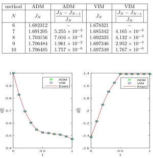
To analysis the accuracy and effectiveness of the ADM and VIM, the rel-ative error of objective value is summarized in Table1, for several iterations. Accordingly, results show that inN = 10, ADM converges to the exact solu-tion. The optimal value of the cost functional is obtained asJ10= 1.706485.
We compared the results obtained from ADM and VIM with exact solu-tion. Figure1 shows the simulation curves ofu(t) at iteration time 10 and the corresponding state trajectory x(t). Results of both methods are very close to exact solution as shown by Figure1. This confirms that the proposed method yields excellent results.
Galley
Pro
of
Table 1: Simulation results of Example 1 at different iteration times.
method ADM ADM VIM VIM
N JN
JN −JN−1
JN
JN
JN −JN−1
JN
6 1.682312 − 1.678321 −
7 1.691205 5.255×10⁻² 1.685342 4.165×10⁻² 8 1.703156 7.016×10⁻² 1.692335 4.132×10⁻³
9 1.706484 1.961×10⁻² 1.697346 2.952×10⁻³
10 1.706485 1.757×10⁻⁶ 1.697349 1.767×10⁻⁶
t
0 0.5 1
u(t)
-2.6 -2.4 -2.2 -2 -1.8 -1.6 -1.4
ADM VIM Exact
t
0 0.5 1
x(t)
0.4 0.5 0.6 0.7 0.8 0.9 1
ADM VIM Exact
Figure 1: The suboptimal control and state, whenN= 10 for Example 1.
˙
x(t) =−x(t) +x(t−1
3) +u(t)− 1 2u(t−
2
3), 0⩽t⩽1, x(t) = 1, −1
3 ⩽t⩽0, u(t) = 0, −2
3 ⩽t⩽0,
(37)
with the cost functional
J =1 2
∫ 1
0
(
x2(t) +1 2u
2(t)
)
(t)dt. (38)
According to system (1), we have A =−1, A1 =B = 1, B1 =−12, Q =
1, R=12.
Galley
Pro
of
results at different iteration times are summarized in Table 2. From Table
2, it is observed that convergence is achieved after 10 iterations, that is,
J10−J9
J10
= 8.040×10⁻⁷<8.1×10⁻⁷.
In Table3, the minimums ofJ using the hybrid of block pulse and Leg-endre polynomials [21], hybrid of general block pulse and Legendre polyno-mials [36], orthogonal basis [16], hybrid of block pulse and orthogonal Taylor series [7], and present two methods are listed. Also the suboptimal control and state of the proposed ADM and VIM are demonstrated in Figure2.
Table 2: Simulation results of Example 2 at different iteration times
method ADM ADM VIM VIM
N JN
JN −JN−1
JN
JN
JN −JN−1
JN
6 0.36430512 − 0.35935108 −
7 0.36512980 2.258×10⁻² 0.36431299 1.382×10⁻²
8 0.37311212 2.139×10⁻² 0.37511283 2.879×10⁻²
9 0.37311294 2.519×10⁻⁶ 0.37311210 5.362×10⁻³
10 0.37311291 8.040×10⁻⁷ 0.37311310 2.680×10⁻⁶
Table 3: The cost functional values for Example 2
Method Cost functional values
Marzban and Razzaghi [21] 0.37311241
Wang [36] 0.37312682
Kellat [16] 0.3731123
Dadkhah and Farahi [7] 0.373112935 Proposed method (N = 10)
ADM 0.37311291
VIM 0.37311310
Example 3. Consider the following linear time-varying multi-delay systems [12,18,23]:
˙
x1(t) =x2(t) +x1(t−1), t≥0,
˙
x2(t) =tx1(t) + 2x1(t−1) +x2(t−1) +u(t)−u(t−0.5),
x1(t) =x2(t) = 1, −1⩽t⩽0,
u(t) = 5(t+ 1), −0.5⩽t⩽0,
(39)
Galley
Pro
of
t
0 0.5 1
x(t)
0.6 0.65 0.7 0.75 0.8 0.85 0.9 0.95 1
ADM VIM
t
0 0.5 1
u(t)
-1 -0.9 -0.8 -0.7 -0.6 -0.5 -0.4 -0.3 -0.2 -0.1 0
ADM VIM
Figure 2: The suboptimal control and state, whenN= 10 for Example 2.
J =1 2x
2 1(3) +x
2 2(3) +
1 2
∫ 3
0
[2x21(t) + 2x1(t)x2(t) +x22(t) +
u2(t)
(t+ 2)]dt. (40)
According to system (1), we have A=
( 0 1 t 0 )
, A1=
( 1 0 2 1 )
, B=
( 0 1 )
, B1=
( 0 −1
)
,
and from (2), we get Qf =
( 1 0 0 2 )
, Q=
( 2 1 1 1 )
, R= 1/(t+ 2).
In order to obtain an accurate enough suboptimal control law, we applied the proposed algorithm with the tolerance bounds ϵ = 2.3×10⁻⁶.
Simu-lation results at different iteration times are summarized in Table 4. From Table 4, it is observed that convergence is achieved after 12 iterations, that is, J12−J11
J12
= 2.270×10⁻⁶<2.3×10⁻⁶. Table 5, a comparison is made
Galley
Pro
of
Table 4: Simulation results of Example 3 at different iteration times
method ADM ADM VIM VIM
N JN
JN −JN−1
JN
JN
JN −JN−1
JN
8 23.21056 − 22.17650 −
9 23.05198 6.879×10⁻² 22.15431 1.001×10⁻² 10 22.02108 1.681×10⁻³ 22.01430 5.903×10⁻³
11 22.02230 5.539×10⁻⁵ 22.02143 3.237×10⁻⁴
12 22.02235 2.270×10⁻⁶ 22.02115 1.271×10⁻⁵
Table 5: The cost functional values for Example 3
Method Cost functional values
Malek-Zavarei [18] 24.0200500
Hwang and Chen [12] 22.0212
Marzban and Pirmoradian [23] 22.0230201080 Proposed method (N = 12)
ADM 22.02235
VIM 22.02115
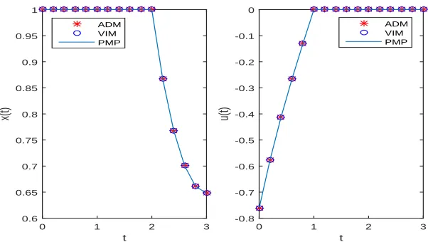
Example 4. We now consider the following nonlinear time-varying multi-delay systems:
˙
x(t) =x(t−1)x(t−2)u(t−2), 0⩽t⩽3, x(t) = 1, −2⩽t⩽0,
u(t) = 0, −2⩽t⩽0,
(41)
with the cost functional
J = ∫ 3
0
(x2(t) +u2(t))dt. (42)
This optimal control is adopted from [10,34,35]. In order to obtain an accu-rate enough suboptimal control law, we applied the proposed algorithm with the tolerance boundsϵ= 1.2×10⁻⁶. Table6, a comparison is made between
Galley
Pro
of
Table 6: The cost functional values for Example 4
Method Cost functional values
Wachter et al. [35](600 grid points) 2.763044 Vanderbei [34](600 grid points) 2.763044 Gollmann et al. [10](600 grid points) 2.761594156
Proposed method (N = 13)
ADM 2.761591012
VIM 2.761592238
t
0 1 2 3
x(t)
0.6 0.65 0.7 0.75 0.8 0.85 0.9 0.95 1
ADM VIM PMP
t
0 1 2 3
u(t)
-0.8 -0.7 -0.6 -0.5 -0.4 -0.3 -0.2 -0.1 0
ADM VIM PMP
Figure 3: The suboptimal control and state, whenN= 13 for Example 4.
6 Conclusion
Galley
Pro
of
Acknowledgements
Author is grateful to the anonymous referees and the editors for their con-structive comments.
References
1. Adomian, G. Nonlinear stochastic systems theory and applications to physics, Kluwer Academic Publishers, 1989, Boston.
2. Adomian, G.A review of the decomposition method in applied mathemat-ics, J. Math. Anal. Appl. 135(2) (1989), 501–544.
3. Alizadeh, A. and Effati, S.Numerical schemes for fractional optimal con-trol problems, J. Dyn. Sys. Meas. Contr. 4 (2017), 1–14.
4. Balasubramaniam, P., Krishnasamy, R. and Rakkiyappan, R. Delay-dependent stability of neutral systems with time-varying delays using delay-decomposition approach, Appl. Math. Model. 36 (2012), 2253–2261.
5. Banks, H.T. and Burns, J.A.Hereditary control problem: Numerical meth-ods based on averaging approximations, SIAM J. Contr. Optim. 16(2) (1978), 169–208.
6. Basin, M. and Rodriguez-Gonzalez, J. Optimal control of linear systems with multiple time delays in control input, IEEE Trans. Automat. Contr. 51(1) (2006), 91–97.
7. Dadkhah, M. and Farahi, M.H.Optimal control of time delay systems via hybrid of block-pulse functions and orthogonal Taylor series, Int. J. Appl. Comput. Math. 2(1) (2016), 137–152.
8. Edrisi-Tabriz, Y., Lakestani, M. and Heydari, A. Two numerical methods for nonlinear constrained quadratic optimal control problems using linear B-spline functions, Iranian J. Numer. Anal. Optim. 6(2) (2016), 17–37.
9. Gollmann, L., Kern, D. and Maurer, H. Optimal control problems with delays in state and control variables subject to mixed control state con-straints, Optim. Contr. Appl. Meth. 30 (2009), 341–365.
10. Gollmann, L. and Maurer, H.Theory and applications of optimal control problems with mul-tiple time delays, J. Ind. Manag. Optim. 10(2) (2014), 413–441.
Galley
Pro
of
12. Hwang, G. and Chen, M.Y. Suboptimal control of linear time-varying multi-delay systems via shifted Legendre polynomials, Int. J. Syst. Sci. 16(12) (1985), 1517–1537.
13. Jajarmi, A., Dehghan-Nayyeri, M. and Saberi-Nik, H. A novel feedforward-feedback suboptimal control of linear time-delay systems via shifted Legendre polynomials, J. Complex. 35 (2016), 46–62.
14. Jamshidi, M. and Wang, C.M.A computational algorithm for large-scale nonlinear time-delays systems, IEEE Trans. Syst. Man. Cyber. SMC. 14 (1984), 2–9.
15. Kharatishvili, G.L.The maximum principle in the theory of optimal pro-cess with time-lags, Doklady Akademii Nauk SSSR. 136 (1961), 39–42.
16. Khellat, F. and Vasegh, N. Suboptimal control of linear systems with delays in state and input by orthogonal basis, Int. J. Comput. Math. 88(4) (2011), 781–794.
17. Koshkouei, A.J., Farahi, M.H. and Burnham, K.J. An almost optimal control design method for nonlinear time-delay systems, Int. J. Contr. 85(2) (2012), 147–158.
18. Malek-Zavarei, M.Near-optimum design of nonstationary linear systems with state and control delays, J. Optim. Theor. Appl. 30 (1980), 73–88.
19. Marzban, H.R. Optimal control of linear multi-delay systems based on a multi-interval decomposition scheme, Optim. Contr. Appl. Meth. 37(1) (2016), 190–211.
20. Marzban, H.R. and Hoseini, S.M.An efficient discretization scheme for solving nonlinear optimal control problems with multiple time delays, Op-tim. Contr. Appl. Meth. 37(4) (2016), 682–707.
21. Marzban, H.R. and Razzaghi, M.Optimal control of linear delay systems via hybrid of block-pulse and Legendre polynomials, J. Franklin Inst. 341 (2004), 279–293.
22. Marzban, H.R. and Pirmoradian, H.A direct approach for the solution of nonlinear optimal control problems with multiple delays subject to mixed state-control constraints, Appl. Math. Model. 53 (2018), 189–213.
23. Marzban, H.R. and Pirmoradian, H. A novel approach for the numer-ical investigation of optimal control problems containing multiple delays, Optim. Contr. Appl. Meth. 39(1) (2018), 302–325.
Galley
Pro
of
25. Mirhosseini-Alizamini, S.M. Numerical solution of the controlled har-monic oscillator by homotopy perturbation method, Contr. Optim. Appl Math. 2(1) (2017), 77–91.
26. Mirhosseini-Alizamini, S.M. and Effati, S. An iterative method for sub-optimal control of a class of nonlinear time-delayed systems, Int. J. Contr. 92 (12) (2019), 2885–2869.
27. Mirhosseini-Alizamini, S.M., Effati, S. and Heydari, A. An iterative method for suboptimal control of linear time-delayed systems, Syst. Contr. Lett. 82 (2015), 40–50.
28. Mirhosseini-Alizamini, S.M., Effati, S. and Heydari, A. Solution of lin-ear time-varying multi-delay systems via variational iteration method, J. Math. Comput. Sci. 16 (2016), 282–297.
29. Nazemi, A. and Mansoori, M. Solving optimal control problems of the time-delayed systems by Haar wavelet, J. Vib. Contr. 22(11) (2014), 2657– 2670.
30. Nazemi, A. and Shabani, M.M. Numerical solution of the time-delayed optimal control problems with hybrid functions, IMA J. Math. Contr. In-form. 32(3) (2015), 623–638.
31. Richard, J.P.Time-delay systems: An overview of some recent advances and open problems, Automatica, 39 (2003), 1667–1694.
32. Saberi Nik, H., Rebelo, P. and Zahedi, S. Solution of infinite horizon nonlinear optimal control problems by piecewise Adomian decomposition method, Math. Model. Anal. 18(4) (2013), 543–560.
33. Shehata, M.M. A study of some nonlinear partial differential equations by using Adomian decomposition method and variational iteration method, Am. J. Comput. Math. 5 (2015), 195–203.
34. Vanderbei, R.J. and Shanno, D.F. An interior-point algorithm for non-convex nonlinear programming, Comput. Optim. Appl. 13 (1999), 231–252.
35. Wachter, A. and Biegler, L.T.On the implementation of an interior-point filter line-search algorithm for large-scale nonlinear programming, Math. Program. 106 (2006), 25–57.