A Neural Network Method Based on Mittag-Leffler Function for Solving a Class of Fractional Optimal Control Problems

AUT J. Model. Simul., 50(2) (2018) 211-218 DOI: 10.22060/miscj.2018.14448.5106

A Neural Network Method Based on Mittag-Leffler Function for Solving a Class of

Fractional Optimal Control Problems

S. Ghasemi* _{, A.R. Nazemi}

Faculty of Mathematical Sciences, Shahrood University of Technology, Shahrood, Iran

ABSTRACT: In this paper, a computational intelligence method is used for solution of fractional optimal control problems (FOCPs) with equality and inequality constraints. According to the Ponteryagin minimum principle (PMP) for FOCP with fractional derivative in the Riemann- Liouville sense and by constructing a suitable error function, we define an unconstrained minimization problem. In the optimization problem, we use trial solutions for the states, Lagrange multipliers and control functions where these trial solutions are constructed by a feed-forward neural network model. We then minimize the error function using a numerical optimization scheme where weight parameters and biases associated with all neurons are unknown. Examples are included to demonstrate the validity and capability of the proposed method. The strength of the proposed method is its equal applicability for the integer-order case as well as fractional order case. Another advantage of the presented approach is to provide results on entire finite continuous domain unlike some other numerical methods which provide solutions only on discrete grid of point.

Review History: Received: 15 May 2018 Revised: 2 October 2018 Accepted: 27 November 2018 Available Online: 5 December 2018

Keywords:

Ponteryagin minimum principle fractional optimal control problem artificial neural network equality and inequality constraints optimization

1- Introduction

Fractional calculus is the study of integrals and derivatives of real or complex order which returns to the end of the seventeenth century . The theory of integral and derivative was mainly developed in the last three decades of the nineteenth century. Its historical survey, subject terms, detail theory and applications can be found in books by Oldham and Spanier [1], Miller and Ross [2], Samko et al. [3] and Anatoly et al. [4]. Since fractional-order models are usually more appropriate to describe physical systems than conventional integer order models (see [5]-[8]) , there is a growing interest in this area during the last few decades. For example, it has been shown that materials with memory and hereditary effects and dynamical processes including gas diffusion and heat conduction in fractal porous media can be more adequately modeled by fractional-order models [9].

A fractional dynamical system is a system whose dynamics is described by fractional differential equations (FDEs). If FDEs contain a control variable and a performance index is given, we obtain a FOCP that is interesting in fractional systems. Some analytical and numerical methods have been obtained for approximating the FOCP in [10–18] and the references therein. Among the numerical methods , authors in [14] present a general formulation and solution scheme based on finding the numerical solution of the Hamilton-Jacobi-Bellman equation by the Legendre– Gauss collocation method . In [15], for solving a class of FOCPs , the variational iteration method is used . In this work , new Lagrange multipliers are determined and some new iterative formulas are presented . In [18] , a numerical method for solving FOCP’s using Haar wavelets is studied . Although these

methods provide good approximations to the solution, they require a discretization of domain via meshing, which may be challenging in two- or higher dimension problems. The approximate solution derivatives are discontinuous and can seriously impact on the stability of the solution. For obtaining satisfactory accuracy, it may be necessary to deal with finite meshes that significantly increase the computational cost. Some numerical methods also use the operational matrices for solving FOCPs (see [18-20]) ; however , finding the operational matrices is usually difficult and these matrices with high dimensions cause complexity in computations . One promising approach for overcoming these limitations is to employ artificial neural networks based on a network topology, a connection pattern, neural activation properties, train strategy and ability to process data.

There are many references in theory and applications , modeling , design , structure and mathematics of neural networks (see [21-23]) . In particular , the numerical solution of ordinary and partial differential equations [24-28] , optimal control problems [29-32], and numerical solutions of FOCP and FDE [10, 11, 33]. Among these references , authors in10] ] present a numerical technique for FOCPs based on a neural network scheme . The fractional derivative is in the Riemann-Liouville sense and is approximated using the Grunwald-Letnikov (G-L) definition for numerical computation . In [32], a class of nonlinear optimal control problems with inequality constraints is considered. Based on Karush–Kuhn–Tucker optimality conditions of nonlinear optimization problems and by constructing an error function, authors define an unconstrained minimization problem. In [33], the solution of fractional differential equations with delay using a new approach based on artificial neural networks is approximated.

Authors in [33] consider fractional differential equations of variable order with the Mittag-Leffler kernel in the Liouville-Caputo sense.

Investigating a general form of FOCPs with inequality constraints and transforming the inequality constraints in the optimality conditions into a system of nonlinear complementarity problem (NCP) functions is one of the motivations of our research . The other motivation of this research is to inrtroduce a new technique for some types of FOCPs by means of a combination of the Mittag-Leffler function and artificial neural networks that so far has not been utilized for the FOCPs . By obtaining an error function and introducing it as a Lyapunov function in the neural network structure, we can prove the stability and convergence of the method similar to one in [10]. On the other hand , the main advantage of the neural network methods is that they involve a single independent variable regardless of the dimension of the problem . The solutions obtained from the neural network schemes are differentiable and in closed analytical form . Motivated from the above discussion, in this paper we use an indirect method for our numerical method . One of the best properties of the indirect schemes is the high credit of the obtained approximate solution of the main FOCPs . This technique is based on satisfying the first-order of the necessary conditions of FOCPs that originate from calculus of variation and PMP [34] . A general formulation for FOCPs was extended in [35, 36] , where the necessary conditions of the optimization are achieved with the Caputo and Riemann-Liouville derivatives . After imposing PMP on the considered FOCPs , we obtain a two-point boundary value problem (TPBVP) . For solving the TPBVP , we generalize a new collocation method which is based on neural networks as an exciting form of artificial intelligence .

The rest of this paper is organized as it follows. In Section 2, we review some basic definitions and results on fractional calculus. In Section 3, we introduce fractional optimal control problem and explain PMP. In Section 4, the basic idea for discretization and optimization of the problem is provided . Numerical simulations are presented in Section 5, and finally Section 6 includes a brief summary and the conclusion .

2- Preliminaries from Fractional Derivatives and Integrals

Now, it is necessary to introduce some definitions and relations in fractional calculus [3] which are used in this paper.

Definition 2.1. Let f a b: ,

[ ]

→_, α>0 be the order of the integral or the derivative, and n=

[ ]

α +1. For t a b∈

[ ]

, , we define:

I. the left and right Riemann-Liouville fractional integral, respectively by

( )

_{( ) (}

)

1

( )

(

)

1 , ,

t

a t

a

I f tα t _τ α f _{τ τ}d t a

α

−

= − >

Γ

∫

(1)

( )

_{( ) (}

)

1

( )

(

)

1 , ,

b

t b

t

I f tα _τ t α f _{τ τ}d t b

α

−

= − <

Γ

∫

(2)

II. the left and right Riemann-Liouville fractional derivatives, respectively by

( )

₍

₎

(

)

1

( )

(

)

1 ( ) , ,

t n n a t a d

D f t t f d t a

n dt

α

α _{τ τ τ}

α

− −

= − >

Γ −

∫

(3)

( )

( )

₍

₎

(

)

1

( )

(

)

1n _{( )} b _{, ,} n

n t b

t d

D f t t f d t b

n dt α α _{τ τ τ} α − − −

= − <

Γ −

∫

(4)

III. the left and right Caputo fractional derivatives of f t

( )

of order α, respectively by

( )

₍

_{) (}

)

1 ( )

_{( )}

₍

₎

1 , ,

t

n n

C a t

a

D f t t f d t a

n

α

α _{τ τ τ}

α

− −

= − >

Γ −

∫

(5)

( )

( )

₍

_{) (}

)

1 ( )

_{( )}

₍

₎

1 , , n b n n C t b t

D f t t f d t b

n α α _{τ τ τ} α − − −

= − <

Γ −

∫

(6)

where _f( )n

( )

_{τ is the usual derivative of f}

( )

_{τ with order n.}

The following relations show the connection between Caputo and Riemann-Liouville fractional derivatives,

( )

( )

1

₍

( )

( )

_{) (}

)

0 , 1 n n _k C

a t a t

k

f a

D f t D f t t a

k α α α α − ₋ = = − − Γ + −

∑

(7)

( )

( )

1

₍

( )

( )

_{) (}

)

0 . 1 n n k C

t b t b

k

f b

D f t D f t b t

k α α α α − − = = − − Γ + −

∑

(8)

Where 0<α<1, we have

( )

( )

₍

( )

_{) (}

)

₁

,

C

a t a t

f a

D f t

α

D f t

α

t a

α

α

−

=

−

−

Γ −

( )

( )

₍

( )

_{) (}

)

₁

.

C

t b t b

f b

D f t

α

D f t

α

b t

α

α

−

=

−

−

Γ −

(9)

The Riemann-Liouville fractional derivative of the exponential function _{f t}

( )

_=eat _{is given by}

( )

0

D e

tα at

=

t M

−α 1,1−α

at

,

(10)

where M_1,1−α

_{( )}

at is the Mittag-Leffler function of two

parameters β =1, and γ = −1 α is defined by the series expansion

( )

₍

₎

(

)

,

0

, 0, 0 .

k k t M t k β γ _{β γ} β γ ∞ =

= > >

Γ +

∑

(11)

3- Mathematical Modeling of the Problem

Consider the FOCP as

(

)

0

minimize J=

_∫

bL t x u dt, , , (12)

( )

( )

(

)

(

)

( )

0 0 , , , subject to , , 0,

0 ,

t

Ax t B D x t F t x u G t x u

x x α  + =  _≤   ₌   (13)

where _{x t}

( )

_∈p _{is the state variable, u t}

_{( )}

_∈q _{is the control}

variable and t∈. It is assumed that the integrand L has continuous first and second partial derivatives with respect to all its arguments. In addition, we assume that F is Lipschitz continuous on a set _{Ω ⊆}p_{. Also α is given a real positive}

constant. According to discussions in [32, 36], if

( )

x u, be a minimum solution of (12) and (13), then there exist λ

( )

t and

( )

t

µ which

(

x u, , , λ µ

)

satisfies

( )

t b

( )

H

(

, , , , ,

)

A t B D t t x u

x

α

λ − λ = −∂ λ µ

∂

( )

0 t

( )

H

(

, , , , ,

)

Ax t B D x tα t x u _{λ µ}

λ

∂

+ =

∂

 ₍₁₅₎

(

, , , ,

)

0,

H t x u

u λ µ

∂ ₌

∂ (16)

(

, ,

)

0,

G t x u

µ = (17)

0,µ> (18)

(

, , 0,

)

G t x u ≤ (19)

( )

0 0,

( )

0,

x =x λ b = (20)

where H denotes the Hamiltonian and is defined in the form of

(

, , , ,

)

(

, ,

)

(

, ,

)

(

, , .

)

H t x uλ µ =L t x u +λF t x u +µ t x u

We can establish the relationship between the solution to nonlinear complementarity problem (NCP) (17)-(19) and the solution to an equivalent equation using an NCP function (see [37]). The class of NCP-functions defined below is used to construct an interesting property.

Definition 3.1. [37] A function _ϕ:2_{→ is called an}

NCP-function if it satisfies

( )

a b, 0 a 0, 0, b ab 0.

ϕ = ⇔ ≥ ≥ =

A popular NCP-function is the Fischer-Burmeister (FB) function, which is strongly semi-smooth and is defined as

(

)

2 2_.

FB a b a b

ϕ = + − +

The perturbed FB function is also given by

(

)

2 2 _{, 0 .}

FBε a b a b

ϕ = + − + +ε ε→ +

The important property of ϕFBε is stated by the following

proposition.

Proposition 3.1. [37] For every ε ∈ _ we have

( )

, 0 0, 0, . 2

FBε a b a b ab

ε

ϕ = ⇔ > > =

Using the perturbed FB function, we can thus convert the

NCP (17)-(19) into equality constraints as

(

)

(

, , ,

)

0, 0 .

FB G t x u

ε

ϕ µ − = ε→ ₊

Therefore, the system (14)-(20) can be rewritten in the following form,

( )

( )

(

)

( )

( )

(

)

(

)

(

)

(

)

( )

( )

0

0

, , , , , , , , , , , , , , 0,

, , , 0, 0 , 0 , 0.

t b

t

FB

H

A t B D t t x u

x H

Ax t B D x t t x u

H t x u u

G t x u

x x b

α

α

ε

λ λ λ µ

λ µ λ

λ µ

ϕ µ ε

λ

+

∂

 _{− = −}

 _∂



∂

 _{+ =}

 _∂

∂

 ₌

 ∂ 

 _{− = →}



 = =

 





(21)

4- Discretization and Optimization

In this section, we provide the introductory materials for the mathematical modeling of system (21) with feed-forward artificial neural network [38]. We can establish the relationship between the solution to the optimality conditions (21) and the solution to an equivalent unconstrained minimization problem via the trial solutions. These trial functions for the state, Lagrangian multipliers, and control functions are selected as

( )

( )

( )

( )

1

1

1

1

, , ,

,

,

,

, .

I

x x x x x

T i i i i i

i_I

T i i i i i

i_I

T i i i i i

i I

u u u u u

T i i i i i

i

x v z z w t b

v z z w t b

v z z w t b

u v z z w t b

λ λ λ λ λ

µ µ µ µ µ

σ

λ σ

µ σ

σ

= = = =





= = +

= = +

= = +

= = +

∑

∑

∑

∑

        

(22)

where I is the number of neurons that can be different for each neural network; w v, are the weight parameters, and b

represents the bias. Also, σ is the exponential function _ex _as

a candidate to replace the log-sigmoid function in the neural network model. It has a universal function approximating

capability and known fractional derivative as well. A generic form of the neural network architecture for FOCPs is represented in Figure 1.

The approximate continuous mappings in the form of linear combination of exponential functions can be taken to approximate the solution x_T, , , λ µ_{T T} u_T and its integer and fractional derivatives. The trial solutions in (22) must satisfy in conditions (21). We thus have

( )

( )

(

, , , ,

)

,

T t b T T T T T

T H

A t B D t t x u

x

α

λ − λ = −∂ λ µ

∂

 ₍₂₃₎

( )

0

( )

(

, , , ,

)

,

T t T T T T T

T H

Ax t B D x tα t x u _{λ µ}

λ ∂

+ =

∂

 ₍₂₄₎

(

, , , , T T T T

)

0,

T H t x u

u λ µ

∂ ₌

∂ (25)

(

)

(

, , ,

)

0, 0 ,

FBε T G t x uT T

ϕ µ − = ε→ _{+ (26)}

( )

0 0,

( )

0.

T T

x =x λ b = (27)

In order to reformulate (23)-(27) as an unconstrained minimization problem, we first collocate the optimality system (23)-(27) on m+1 points t k_k, 0,1 , , = …m, of the interval

[ ]

a b, . According to (10) and the introduced structure of the neural network in the exponential form, an approximation of the left Riemann- Liouville fractional derivative ₀D x t_tα _T

( )

in (24) is easily computable in the following form,

( )

( )

0 1, 1

0 . i I b x x

t T i i

i

D x tα v e t Mα w t

α

− − =

=

∑

For the right Riemann-Liouville fractional derivative

( )

tDb Tαλ t in (23), by using the equations

(6) and (8), it is desirable to use its equivalent form as it follows,

( )

₍

( )

_{) (}

)

₍

_{) (}

)

( )

_{1 1}1 .

b T

t b T T

t

b

Dα_λ t λ b t α _τ t α_{λ τ τ}d

α α

− −

= − − −

Γ − Γ −

∫

 (28)

We can approximate integral in (28) by any numerical integration techniques such as Simpson rule [39]. We now define an optimization problem as

( )

( ) ( ) ( ) ( ) ( ) ( )

{

1 2 3 4 5 6

}

0 minimize

1 _{, , , , , ,}

2

y m

k k k k k k

k

E y

E t y E t y E t y E t y E t y E t y

=

=

+ + + + +

∑

(29)

where

(

_{, , , , , , , , , , ,}

)

4 3I p q( )

x u x u x u

y= w w w w b b b b v v v vλ µ λ µ λ µ ∈R + and

( ) ( ) ( ) ( ) ( ) ( ) ( ) ( ) ( ) ( ) 2 1 2 2 0 3

, , , , , , 0,1 , , 1,

, , , , , , 1, 2, , ,

, , , , ,

k T t b T T T T T

k t T T T T T

k T T T T

H

E t y Ax t B D t t x u k m

x H

E t y A t B D x t t x u k m

H

E t y t x u

u α α λ λ µ λ λ µ λ λ µ ∂   =_ − + _ = … − ∂   ∂   =_ + − _ = … ∂   ∂   =  ∂   ( ) ( ( )) ( ) ( ) 2 2 4 2 5 0

, 1, 2, , , , , , , , 1, 2, , , , 0 ,

k FB T T

k T

k m

E t y G t x u k m

E t y x x

ε ϕ µ = …    =_ − _ = … =_ − _

( ) ( )2 6

1, 2, , , , , 1, 2, , .

k T

k m

E t y λ b k m

              = … = = …    (30)

Lemma 4.1. [10] If:

(

)

* *_{, , , , , , , , , , ,} * * * * * * * * * * *

x u x u x u

y = w w w w b b b b v v v vλ µ λ µ λ µ

satisfies the equality

( )

(

)

(

)

(

)

(

)

(

)

(

)

(

)

(

)

(

)

(

)

(

)

(

)

1 1 1 2 1 2 3 1 3 4 1 4 5 1 5 6 1 6 , , , , , , 0 , , , , , , m m m m m m E t y

E t y E t y

E t y E t y

E t y y

E t y

E t y E t y

E t y E t y

E t y

γ                               =_{ }=                                     (31)

then _y* _{is an optimal solution of (29).}

Proof. Let _γ

( )

_y* _{=0. Then for i= …1, 6 and k= …1, , m,}

we have

(

_, *

)

₀

i k

E t y = . Since in (29) E y

( )

≥0, thus _y* _is

an optimal solution of (29).

By Lemma 4.1, we can easily verify that the minimization problem (29) is equivalent to the following problem,

( )

1

( )

2

minimize . 2

y E y = γ y (32)

In order to solve the unconstrained optimization problem in (32), we can use any optimization algorithms such as the steepest descent, Newton, quasi-Newton, conjugate gradient, etc. [40-42] and the heuristic algorithms such as genetic algorithm, particle swarm optimization, ant colony search algorithms, etc. [43].

5- Numerical Examples

In this section, we try to implement two numerical examples to illustrate the efficiency and applicability of the proposed method.

Example 5.1. We consider a single-input scalar system as follows,

( )

( )

(

)

1 2 2 0 1

minimize , 2

J=

∫

x t +u t dt

( )

( ) ( )

0

subject to D x t_tα _{= −}x t u t₊ ,

with the initial condition x

( )

0 =0. The analytical solution of the mentioned problem with α =1 _{is given in [36] as}

( )

cosh 2

( )

sinh 2 ,

( )

x t = t +β t

( )

(

) ( ) (

) ( )

u t = +1 2 cosh 2β t + 2+β sinh 2 ,t

where

( )

( )

( )

( )

cosh 2 2 sinh 2

0.98. 2 cosh 2 sinh 2

t t

t t

β= − + ≈ −

According to (21) we have

( ) ( ) ( )

( )

( ) ( )

( ) ( )

( )

( )

1

0

, , 0, 0 1, 1 0.

t

t

D t x t t

D x t x t u t

u t t

x

α α

λ λ

λ λ

 = −

 _{= − +}



 _{+ =}



 = =



Since x

( )

1 is free, we have λ

( )

1 0= . Corresponding to this condition and the initial condition x

( )

0 1= , we choose the trial solutions as

( )

( )

1

1

1

,

,

,

0

0, 1 0.

x x

i i

i i

u u i i

I

w t b x

T i

i I

w t b

T i

i I

w t b u

T i

i

T T

x

v e

v e

u

v e

x

λ λ

λ

λ

λ

+

=

+

=

+

=



₌







=







 =





₌

₌



∑

∑

∑

We obtain the approximate solution of state and control functions by using the presented method in the cases of

1

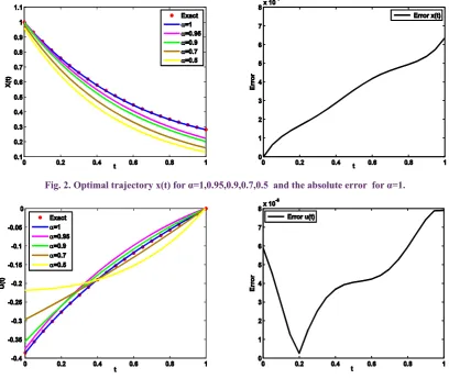
α = and several values of α. In Figures 2 and 3, the exact solutions for α =1, approximate solutions of the neural network scheme for α=1, 0.95, 0.9, 0.7, 0.5 and the absolute error for α =1 are shown for the state and control functions, respectively.

Example 5.2. In the second example, we consider an

optimization problem with inequality constraints as it follows,

( )

1

0

minimize

_∫

u t dt,

( ) ( )

( )

( )

( )

( ) ( )

0 ,

0 1, 1 ,

subject to 0,

0.

C t

D x t u t

x x is free

u t x t u t

α

 =

 ₌



 _≥



 − ≥



The exact state and control functions for α =1 are

( )

exp

( )

x t = t and u t

( )

=exp

( )

t (see [32]). Since x

( )

1

is free, we have λ

( )

1 0= . Corresponding to this condition and the initial condition x

( )

0 1= , we can choose the trial solutions as

( )

( )

1 1

2 2

1

1

1

1 1

1

2 2

1

,

, ,

, 0 0, 1 0

,

.

x x i i

i i

u u i i

i i

i i

I w t b x

T i

i I

w t b

T i

i I

w t b u

T i

i I

w t b

T i

i I

w t b

T i

i

T T

x v e

v e

u v e

v e

v e

x

λ λ

µ µ

µ µ

λ

µ

µ

λ

µ

µ

λ

+ =

+ =

+ =

+ =

+ =

 =   

=   

=   

 =

 

 =



 _{= =}



∑

∑

∑

∑

∑

Fig. 2. Optimal trajectory x(t) for α=1,0.95,0.9,0.7,0.5 and the absolute error for α=1.

We illustrate the approximate solutions for x t

( )

and u t

( )

in Figures 4 and 5, respectively.

6- Conclusion

This paper presents an indirect method for solving a class of FOCPs based on a combination of the Mittag-Leffler function and artificial neural networks. The discussed problem includes the integer and fractional order derivatives with equality and inequality constraints. In this novel method, the inequality constraints in the optimality conditions are transformed into a system of NCP functions. An approach based on feed-forward neural networks, optimization techniques, and collocation methods is then stated to determine the approximate solution of the FOCPs.

It should be noted that in the method presented in this paper, after obtaining the values of weights by solving the unconstrained optimization problem (32), we put the obtained weights in the trial solutions (22). We then plot the response curve continuously without any need to the use of interpolation or fitting methods [39]. However, in some other numerical methods such as collocation methods, finite element methods, finite difference methods, etc., one acquires first the solution in different points, discretely. One then plots the curve solution by interpolation or fitting methods. This is an important disadvantage of some other methods compared with neural network methods. In fact, the obtained solution by the neural network methods is in a closed analytical form.

References

[1] Oldham K, Spanier J. The fractional calculus theory and applications of differentiation and integration to arbitrary order: Elsevier; 1974.

[2] Miller KS, Ross B. An introduction to the fractional calculus and fractional differential equations. 1993.

[3] Samko S, Kilbas A, Marichev O. Fractional integrals and derivatives and some of their applications. Science and Technica. 1987;1.

[4] Kilbas AAA, Srivastava HM, Trujillo JJ. Theory and applications of fractional differential equations: Elsevier Science Limited; 2006.

[5] Torvik PJ, Bagley RL. On the appearance of the fractional derivative in the behavior of real materials. Journal of Applied Mechanics. 1984;51(2):294-8.

[6] Khader M, Sweilam N, Mahdy A. An efficient numerical method for solving the fractional diffusion equation. Journal of Applied Mathematics and Bioinformatics. 2011;1(2):1.

[7] Oustaloup A, Levron F, Mathieu B, Nanot FM. Frequency-band complex noninteger differentiator: characterization and synthesis. IEEE Transactions on Circuits and Systems I: Fundamental Theory and Applications. 2000;47(1):25-39.

Fig.5. Optimal control u(t) for α=1,0.95,0.9,0.8,0.7 and the absolute error for α=1.

[8] Tricaud C, Chen Y. An approximate method for numerically solving fractional order optimal control problems of general form. Computers & Mathematics with Applications. 2010;59(5):1644-55.

[9] Zamani M, Karimi-Ghartemani M, Sadati N. FOPID controller design for robust performance using particle swarm optimization. Fractional Calculus and Applied Analysis. 2007;10(2):169-87.

[10] Ghasemi S, Nazemi A, Hosseinpour S. Nonlinear fractional optimal control problems with neural network and dynamic optimization schemes. Nonlinear Dynamics. 2017;89(4):2669-82.

[11] Sabouri J, Effati S, Pakdaman M. A neural network approach for solving a class of fractional optimal control problems. Neural Processing Letters. 2017;45(1):59-74.

[12] Tohidi E, Nik HS. A Bessel collocation method for solving fractional optimal control problems. Applied Mathematical Modelling. 2015;39(2):455-65.

[13] Singha N, Nahak C. An efficient approximation technique for solving a class of fractional optimal control problems. Journal of Optimization Theory and Applications. 2017;174(3):785-802.

[14] Rakhshan SA, Effati S, Vahidian Kamyad A. Solving a class of fractional optimal control problems by the Hamilton–Jacobi–Bellman equation. Journal of Vibration and Control. 2018;24(9):1741-56.

[15] Alizadeh A, Effati S. An iterative approach for solving fractional optimal control problems. Journal of Vibration and Control. 2018;24(1):18-36.

[16] Almeida R, Torres DF. A discrete method to solve fractional optimal control problems. Nonlinear Dynamics. 2015;80(4):1811-6.

[17] Pooseh S, Almeida R, Torres DF. Fractional order optimal control problems with free terminal time. arXiv preprint arXiv:13021717. 2013.

[18] Hosseinpour S, Nazemi A. A collocation method via block-pulse functions for solving delay fractional optimal control problems. IMA Journal of Mathematical Control and Information. 2016;34(4):1215-37.

[19] Jafari H, Tajadodi H. Fractional order optimal control problems via the operational matrices of Bernstein polynomials. UPB Sci Bull. 2014;76(3):115-28.

[20] Heydari M, Hooshmandasl MR, Ghaini FM, Cattani C. Wavelets method for solving fractional optimal control problems. Applied Mathematics and Computation. 2016;286:139-54.

[21] Daniel G. Principles of artificial neural networks: World Scientific; 2013.

[22] Tang H, Tan KC, Yi Z. Neural networks: computational models and applications: Springer Science & Business Media; 2007.

[23] Müller B, Reinhardt J, Strickland MT. Neural networks: an introduction: Springer Science & Business Media; 2012.

[24] Beidokhti RS, Malek A. Solving initial-boundary value problems for systems of partial differential equations

using neural networks and optimization techniques. Journal of the Franklin Institute. 2009;346(9):898-913.

[25] Kumar M, Yadav N. Multilayer perceptrons and radial basis function neural network methods for the solution of differential equations: a survey. Computers & Mathematics with Applications. 2011;62(10):3796-811.

[26] Dua V. An artificial neural network approximation based decomposition approach for parameter estimation of system of ordinary differential equations. Computers & chemical engineering. 2011;35(3):545-53.

[27] Shirvany Y, Hayati M, Moradian R. Numerical solution of the nonlinear Schrodinger equation by feedforward neural networks. Communications in Nonlinear Science and Numerical Simulation. 2008;13(10):2132-45.

[28] Shirvany Y, Hayati M, Moradian R. Multilayer perceptron neural networks with novel unsupervised training method for numerical solution of the partial differential equations. Applied Soft Computing. 2009;9(1):20-9.

[29] Vrabie D, Lewis F. Neural network approach to continuous-time direct adaptive optimal control for partially unknown nonlinear systems. Neural Networks. 2009;22(3):237-46.

[30] Cheng T, Lewis FL, Abu-Khalaf M. Fixed-final-time-constrained optimal control of nonlinear systems using neural network HJB approach. IEEE Transactions on Neural Networks. 2007;18(6):1725-37.

[31] Effati S, Pakdaman M. Optimal control problem via neural networks. Neural Computing and Applications. 2013;23(7-8):2093-100.

[32] Nazemi A, Karami R. A neural network approach for solving optimal control problems with inequality constraints and some applications. Neural Processing Letters. 2017;45(3):995-1023.

[33] Zuniga-Aguilar C, Coronel-Escamilla A, Gómez-Aguilar J, Alvarado-Martínez V, Romero-Ugalde H. New numerical approximation for solving fractional delay differential equations of variable order using artificial neural networks. The European Physical Journal Plus. 2018;133(2):75.

[34] Pontryagin L, Boltyanskii V, Gamkrelidze R, Mischenko E. 1964 The mathematical theory of optimal processes. Wiley and Macmillan) English transls. of 1st ed; 1962.

[35] Guo TL. The necessary conditions of fractional optimal control in the sense of Caputo. Journal of Optimization Theory and Applications. 2013;156(1):115-26.

[36] Agrawal OP. A general formulation and solution scheme for fractional optimal control problems. Nonlinear Dynamics. 2004;38(1-4):323-37.

[37] Nazemi A, Nazemi M. A gradient-based neural network method for solving strictly convex quadratic programming problems. Cognitive Computation. 2014;6(3):484-95.

[39] Stoer J, Bulirsch R. Introduction to numerical analysis: Springer Science & Business Media; 2013.

[40] Bazaraa MS, Sherali HD, Shetty CM. Nonlinear programming: theory and algorithms: John Wiley & Sons; 2013.

[41] Zhang X-S. Neural networks in optimization: Springer

Science & Business Media; 2013.

[42] Nocedal J, Wright S. Numerical optimization: Springer Science & Business Media; 2006.

[43] Lee KY, El-Sharkawi MA. Modern heuristic optimization techniques: theory and applications to power systems: John Wiley & Sons; 2008.

Pleasecitethisarticleusing:

S. Ghasemi and A.R. Nazemi, A Neural Network Method Based on Mittag-Leffler Function for Solving a Class of Fractional Optimal Control Problems, AUT J. Model. Simul., 50(2) (2018) 211-218.