in the population sciences published by the Max Planck Institute for Demographic Research Konrad-Zuse Str. 1, D-18057 Rostock · GERMANY www.demographic-research.org
DEMOGRAPHIC RESEARCH
VOLUME 23, ARTICLE 35, PAGES 997-1030
PUBLISHED 19 NOVEMBER 2010
http://www.demographic-research.org/Volumes/Vol23/35/ DOI: 10.4054/DemRes.2010.23.35
Research Article
Income, health, and well-being in
rural Malawi
Brian Chin
This publication is part of the proposed Special Collection “HIV/AIDS in sub-Saharan Africa”, edited by Susan Watkins, Jere Behrman, Hans-Peter Kohler, and Simona Bignami-Van Assche.
© 2010 Brian Chin.
This open-access work is published under the terms of the Creative Commons Attribution NonCommercial License 2.0 Germany, which permits use, reproduction & distribution in any medium for non-commercial purposes, provided the original author(s) and source are given credit.
1 Introduction 998
2 Empirical models 1000
3 Data 1003
3.1 Malawi diffusion and ideational change project (MDICP)/Malawi longitudinal study of families and health (MLSFH)
1003
3.2 Central variables for the analysis 1004
3.2.1 Dependent variables – general health status, subjective well-being, SF-12 scores, and HIV status
1004
3.2.2 Key independent variable – Income 1009
3.2.3 Individual characteristics 1010
3.2.4 Instruments 1011
4 Results 1012
4.1 First-stage regressions 1012
4.2 Second-stage regressions 1013
5 Discussion 1022
6 Acknowledgements 1023
References 1024
Income, health, and well-being in rural Malawi
Brian Chin1
Abstract
This paper attempts to isolate the causal link of income on health status and subjective well-being for the rural population in Malawi using three waves of household panel data spanning the period 2004-2008 from the Malawi Diffusion and Ideational Change Project (MDICP) and the Malawi Longitudinal Study of Families and Health (MLSFH). Malawi is a low-income country with high background morbidity and mortality, as well as an AIDS epidemic, high fertility, and poor reproductive health. Instrumental variables and fixed effects strategies are used to try to address endogeneity of the income to health relationship. The analyses show that a 10% increase in income improves mean general health status of rural Malawians by 1.0% and mean subjective well-being by 1.2%.
1 Population Studies Center, University of Pennsylvania, 3718 Locust Walk, Philadelphia PA 19104,
1. Introduction
Strong causal links may run in both directions between income and health. There is a long literature describing the effects of this endogenous relationship, with examples from the historical decline of mortality in now developed countries as well as the role of economic growth in health improvements in developing countries, recently summarized by Deaton (2006) and Cutler, Deaton, and Lleras-Muney (2006).
McKeown (1979) first emphasized the theory that income, primarily through better nutrition, clothing, and housing, was the primary determinant of health in the history of now rich countries. Detailed data on adult height have been used to support this theory by investigating causes of the historical decline in mortality (Steckel 1995; Fogel 1997, 2004). However, this historical view has been convincingly challenged, most notably by the analyses of Preston (1975; 1980; 1996), Szreter (1988), Guha (1994), and Easterlin (2004), which found that the germ theory of disease and the importance of public health were the main sources of the historical decline in mortality.
The role of economic growth in health improvements in poor countries has also been controversial. Pritchett and Summers (1996) phrased the hypothesis “wealthier is healthier” when they found that economic growth in developingcountries led directly to reductions in infant mortalityrates and improvements in life expectancy. Specifically, they calculated that in 1990 alone, more than half a million child deaths in the developing world could be attributed to poor economic performance in the 1980s. The theory is that improvedhealth was a direct by-product of higher income levels through nutritional factors similarly brought up in the historical account, as well as the fact that higher income enabled provision of infrastructure for public health, such as water and sanitation. Filmer and Pritchett (1999) showed the direct effect of public spending on health, as measured by infant and child (under-5) mortality, was small and explained a small fraction of 1% of the observed differences in mortality across countries. Rather, 95% of cross-national variation in mortality could be explained by non health factors (country’s income per capita, inequality of income distribution, extent of female education, level of ethnic fragmentation, and predominant religion).
studies indicate substantial effects of improved health and nutrition (Alderman, Hoddinott, and Kinsey 2006; Hoddinott et al. 2008).
Despite the disparate findings and theories on the endogenous relationship, the argument that economic growth is by default good for health remains widely accepted, particularly among those arguing for the benefits of globalization and development aid (Filmer and Pritchett 1999; Dollar 2001; World Bank 2002). Until now, there have been only a few studies that have established the causal link between economic resources and health across countries (Pritchett and Summers 1996; Filmer and Pritchett 1999). Given the importance of development and the enormous amount of global economic and health aid committed to resource-poor countries today, it is perhaps surprising that there has not been more systematic analysis of the downstream effect of the income-health causal link at the individual level in, for example, HIV-afflicted regions of Sub-Saharan Africa.
Malawi is a good setting for such a study because it is a very poor country with persistent high TFR, considerable “unmet” family planning needs, high mortality and morbidity, and as in much of south and east Africa, has a mature epidemic with a rural HIV prevalence of 10.8% (National Statistical Office (NSO) [Malawi], and ORC Macro 2005). There has been enormous effort to reduce HIV rates as part of national as well as international development strategic agendas, but without evident success. While the Malawian per capita income is below the Sub-Saharan average, Malawi is similar to other Sub-Saharan African countries and countries in the World Bank low-income group in terms of life expectancy, infant mortality, child malnutrition, access to clean water, literacy, and educational enrollment (World Bank 2009). During the last decade, there has been slow and steady economic growth and associated increases in income in Malawi (African Development Bank and OECD 2009). The effects of these increases in income are ambiguous and largely unknown. For example, HIV risks may go up with income, but some other major health problems such as the major communicable diseases and conditions traditionally associated with poverty (i.e., undernutrition, diarrhea, and maternal health problems) are likely to go down.
millennium, though there have been many important changes since the turn of the century. The development of the MDGs to spur development by improving social and economic conditions in the world’s poorest countries is one example. With this renewed commitment of economic and health aid flowing into countries such as Malawi, it is prudent to focus on more current sources of data.
Much of the academic literature analyzing levels, trends, and determinants of health outcomes and behavior in Sub-Saharan Africa has a focus on HIV, with perhaps an over-emphasis on HIV/AIDS relative to the burden of other diseases (Behrman, Behrman, and Perez 2009). The AIDS literature has ignored, until recently, the potential of individual and familial coping mechanisms for the HIV epidemic; empirical studies by Beegle (2005) and Bignami-Van Assche et al. (forthcoming) have focused on this issue. Moreover, a preponderance of these analyses is based on case studies or cross-sectional surveys that do not permit important distinctions between immediate impacts and longer-term consequences, or lack controls for endowments, unobserved characteristics, behavioral determinants of individual’s and family’s health status, endogenous decision processes, and selective participation in risk prevention efforts. Amidst gripping poverty, the assessments and expectations of one’s own and family members’ health, well-being, and HIV status may influence investments in human and social capital in ways that have not been analyzed before. Therefore, this study contributes to the understanding of the income to health endogenous relationship in a country with vast development challenges, while controlling for the complex linkages between these variables by using time-varying microlevel factors such as rainfall and market prices as instruments in an instrumental variable fixed effects approach applied to three waves of panel data in contrast to the usual cross-sectional aggregate estimates.
2. Empirical models
An empirical specification for the relationship of income determining health can be described as follows. Let H be some health outcome, W be income, and X be a vector of demographic and socioeconomic individual characteristics (e.g., sex, age, marital status, number of children ever born). The effect of income on health is captured by the b coefficient in the regression:
where git are some time-varying unobserved factors that affect both income W and health outcome H for individual i in year t; fi represents unobserved fixed factors (unobserved individual, family, and community characteristics) that are assumed to affect health outcome H; and eit is an independent and identically distributed (i.i.d.) disturbance term.
The outcome variables considered are self-reported measures of health status, subjective well-being, physical and mental health, and HIV status. Income not only improves health directly, but can lead to enhanced food security and improved access to public services, such as water and health services, toward that end. On the reverse side, health is related to income since it can be highly correlated with healthy workers and greater economic productivity. Therefore, the main requirement for consistent estimation of b within a standard regression analysis of Eq. (1), the condition that Cov(Wit, eit | Xit, git)=0, is unlikely to be met. Factors influencing income such as individuals’ expectations regarding future prices and productivity, and interfamilial and community resources on which an individual can draw that may also influence health are not observed and could bias estimates of b because these factors could have a direct effect on health in addition to their effect on income. The estimation of b requires an instrument that predicts income, but, conditional on covariates, is uncorrelated with health. Likewise, it is necessary to eliminate the unobserved time-invariant, individual, family, and community-specific fixed effects fi, and any time-varying unobserved effects git that might affect health as well as income.
Instrumental variables fixed effects (IV-FE) estimation of Eq. (1) can provide a solution to these methodological challenges of identifying the effect b of health on income. In particular, the IV-FE approach is given by
∆Hit = b∆Wit+ a∆Xit+ ∆eit , (2)
The first-stage least squares estimation model is defined as
Wit= k·Zit+ m·Xit + qit+ pi + uit , (3)
where Wit is a measure of income, Zit is a vector of instruments that affects income W but not directly the second-stage health outcome H in Eq. (1), Xit is a vector of individual characteristics, qit are unobserved time-varying factors that affect both instrument(s) Z and income W, pi represents unobserved time-invariant fixed factors, which might be correlated with the fixed unobserved characteristics fi in Eq. (1), that affect an individual’s level of income, and uit are unobserved factors that are uncorrelated with Xitand the second-stage error term eit in Eq. (1).
The fixed effects estimation is applied to Eq. (3) to control for both the time-varying unobserved factors qit and unobserved fixed factors pi that may provide differential comparative advantage in income as described above:
∆Wit= k∆Zit + m∆Xit+ ∆uit . (4)
Omitted variable bias arising from the potential correlation between the instruments Zit and the individual, household, and community-specific time-invariant unobservables pi is adequately addressed by fixed effects since the change in instruments Z must be exogenous. The set of instruments are described in more detail in Section 3.2.4.
3. Data
3.1 Malawi diffusion and ideational change project (MDICP)/Malawi longitudinal study of families and health (MLSFH)
The main source of data used comes from three waves (2004, 2006, and 2008) of the Malawi Diffusion and Ideational Change Project (MDICP) and the Malawi Longitudinal Study of Families and Health (MLSFH), a longitudinal panel survey conducted in Malawi by an ongoing collaborative project between the University of Pennsylvania, the University of Malawi, College of Medicine, and the University of Malawi, Chancellor College. The survey is conducted in three distinctive districts of Malawi: Rumphi (Northern region), Mchinji (Central region), and Balaka (Southern region). Although the sampling strategy was not designed to be representative of the national population of rural Malawi, the sample characteristics closely match those of the rural population of the nationally-representative Malawi Demographic and Health Survey (Bignami-Van Assche, Reniers, and Weinreb 2003; Anglewicz et al. 2009).2 The original wave sampled in 1998 consisted of approximately 1,500 ever-married women ages 15-49, and 1,100 spouses. These respondents were re-interviewed in 2001, and all new spouses of men and women who remarried between 1998 and 2001 were added to the sample. In 2004, in addition to the original sample and their new spouses, approximately 1,500 adolescents and young adults, ages 15-25, some never-married, were added to the sample. In 2006, all respondents from previous waves in 1998, 2001, and 2004 were included in the sample, along with spouses of the adolescents and young adults surveyed in 2004, and any new spouses of respondents in the original sample. In 2008, as with previous waves, all previous respondents and new spouses were included in the study. Also, a new sample of approximately 800 living biological parents of MDICP/MLSFH respondents from 2006 who resided in the same village as the respondent were included. Between 2004 and 2008, approximately 5,300 unique respondents were included with an average number of two surveys. The samples are restricted to nonmissing, nonsingleton (non-one-observation groups) observations for each of the various specifications to maintain constant sample composition. The features of these data that are relevant to the analysis include basic demographic information, household characteristics and assets, consumption expenditures, and a number of health and well-being outcomes. As previously described, the longitudinal nature of the data allows control for unobserved fixed effects. In addition, the data are
2 Detailed descriptions of the MDICP/MLSFH sample selection, data collection, and data quality are provided
on the project website at http://www.malawi.pop.upenn.edu and in a Special Collection of the online journal
comprehensive enough to facilitate causal analyses with instrumental variables and address problems of endogeneity and omitted variable bias in regression analyses as similarly performed by Kohler, Behrman, and Watkins (2007) that examines whether social interactions have a causal effect on HIV/AIDS risk perceptions.
3.2 Central variables for the analysis
3.2.1 Dependent variables – general health status, subjective well-being, SF-12 scores, and HIV status
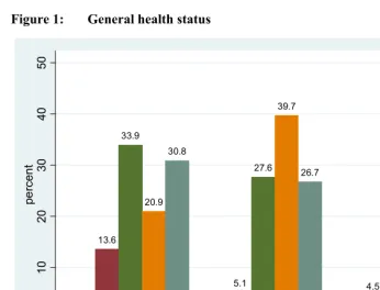
The first dependent variable is self-reported general health status, “In general, would you say your health is: Excellent, Very Good, Good, Fair, or Poor? (1 = Excellent, 2 = Very Good, 3 = Good, 4 = Fair, and 5 = Poor),” which has been used widely in surveys and has been shown to be well correlated with clinical measures of health (Case and Paxson 2005; Case and Wilson 2000).3 Figure 1 shows the distribution of general health status across the three waves. The measures are reported for the same set of persons, and thus differences are due to changes in reported health rather than group composition.From 2004 to 2008, the highest category “Excellent” health decreased 17 percentage points while “Very Good” health increased dramatically by 28.5 percentage points. “Good” health remained fairly constant while “Fair” health decreased 9.1 percentage points. Very few respondents (<1%) reported themselves to be in “Poor” health. Table 1 shows average health status increased from 3.68 to 3.86 between 2004 and 2006, and then decreased to 3.72 in 2008.
The second dependent variable is life satisfaction or subjective well-being, a one-question measure derived from Fordyce (1988) phrased, “I am interested in your general level of well-being or satisfaction with life. How satisfied are you with your life, all things considered? (1 = Very Satisfied, 2 = Somewhat Satisfied, 3 = Satisfied, 4 = Somewhat Unsatisfied, and 5 = Very Unsatisfied).”4 Self-reported subjective well-being consists of an affective part that is a hedonic evaluation guided by emotions and feelings, and a cognitive part that is an information-based appraisal of one’s life for which respondents judge the extent to which their life so far measures up to their expectations and resembles their envisioned “ideal” life (Diener 1994).
3 The variable has been recoded in reverse to enable ease of interpretation, e.g., better health is equivalent to
Figure 1: General health status
0.8 13.6
33.9
20.9 30.8
0.9 5.1
27.6 39.7
26.7
0.3 4.5
31.9 49.4
13.8
0
10
20
30
40
50
pe
rc
en
t
2004 2006 2008
Table 1: Descriptive statistics – means and standard deviations
2004 2006 2008 2004 2006 2008
N 1,180 1,180 1,180 930 930 930
General health status 3.68 3.86 3.72
(1.07) (0.90) (0.77)
Subjective well-being 3.96 4.07
(0.95) (0.94)
PCS-12 52.56 52.31
(7.08) (6.70)
MCS-12 55.57 54.03
(8.41) (8.88)
HIV positive status 0.032 0.039 0.044
(0.177) (0.193) (0.205)
Per capita expenditure 828 900 2,318 836 928 2,446
(2,170) (2,056) (6,992) (2,330) (2,263) (7,737)
Sex 0.35 0.35 0.35 0.36 0.36 0.36
(0.48) (0.48) (0.48) (0.48) (0.48) (0.48)
Age 37.43 39.79 41.66 37.69 40.05 41.85
(11.92) (11.79) (11.84) (11.79) (11.63) (11.64)
(Age/10) squared 15.43 17.22 18.75 15.59 17.39 18.86
(9.70) (10.15) (10.68) (9.66) (10.04) (10.50)
Primary schooling 0.47 0.66 0.67 0.49 0.66 0.67
(0.50) (0.47) (0.47) (0.50) (0.47) (0.47)
Secondary schooling 0.08 0.08 0.08 0.08 0.09 0.09
(0.27) (0.28) (0.28) (0.27) (0.29) (0.29)
Married 0.93 0.93 0.90 0.94 0.94 0.91
(0.26) (0.26) (0.30) (0.23) (0.24) (0.29)
Children ever born 5.73 6.02 6.51 5.77 6.04 6.51
(3.37) (3.20) (3.17) (3.31) (3.15) (3.12)
To the extent that life-satisfaction is guided by an individual’s emotions and feelings, subjective well-being is an indicator to measure mental health. Problems with mental health or depressive disorders are indicated by loss of interest or pleasure, feelings of guilt or low self-worth, disturbed sleep or appetite, low energy, and poor concentration. These in turn can lead to substantial impairments in an individual’s ability to take care of his or her everyday responsibilities. Depression is the leading cause of disability as measured by years lived with disability and the fourth leading contributor to the global burden of disease (DALYs) in 2000 (Üstün et al. 2004).
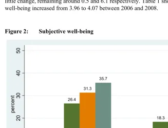
Figure 2 shows the distribution of subjective well-being. From 2006 to 2008, the “Satisfied” category dropped 8.1 percentage points, which resulted in an increase of approximately 4% points for both “Somewhat Satisfied” and “Very Satisfied” categories. The “Very Unsatisfied” and “Somewhat Unsatisfied” categories showed little change, remaining around 0.5 and 6.1 respectively. Table 1 shows mean subjective well-being increased from 3.96 to 4.07 between 2006 and 2008.
Figure 2: Subjective well-being
0.5 6.1
26.4 31.3
35.7
0.5 6.4
18.3 35.3
39.6
0
10
20
30
40
50
pe
rc
en
t
2006 2008
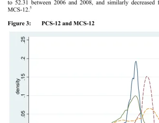
The third and fourth health outcomes come from the health status instrument SF-12 (Ware, Kosinksi, and Keller 2001; 1996), a twelve question composite indicator, derived from its predecessor the SF-36, physical (PCS-12) and mental (MCS-12) health that has been validated globally (including in Sub-Saharan Africa), and is less affected by measurement error than alternative subjective health measures (Dow et al. 1997; Strauss and Thomas 1998).4 Figure 3 is a histogram that shows MCS-12 scores were higher than PCS-12 for both years. Table 1 shows mean PCS-12 decreased from 52.56 to 52.31 between 2006 and 2008, and similarly decreased from 55.57 to 54.03 for MCS-12.5
Figure 3: PCS-12 and MCS-12
0
.0
5
.1
.1
5
.2
.2
5
de
ns
ity
20 40 60 80
score
PCS-12 2006 MCS-12 2006
PCS-12 2008 MCS-12 2008
Notes: Epanechnikov kernel density estimates.
4 For subjective well-being, PCS-12, and MCS-12, data are only available for the 2006 and 2008 waves. 5 SF-12 was used in 2006 and SF-12v2 in 2008. The two sets of questions used are fairly consistent, except
The last heath outcome is HIV status, which is equal to 1 if positive and 0 if negative. The HIV tests were performed for all respondents from the 2004 wave onward according to the protocol by Bignami-Van Assche et al. (2004). Over 90% of respondents in each round accepted the HIVtest, despite variations in testing protocols (Obare et al. 2009). Table 1 shows HIV prevalence increased 1.2 percentage points from 3.2 in 2004 to 4.4 in 2008. The HIV prevalence is lower in the analytical sample when compared to the national rural statistic (10.8%) due in large part to differences in sampling and geographic variation (Obare et al. 2009).
The HIV status variable allows the analysis of how changes in income can directly affect an individual’s HIV status in settings such as rural communities of Sub-Saharan Africa. There is a disagreement in the literature about whether poverty influences HIV/AIDS through multiple environmental and behavioral mechanisms (Halperin and Allen 2000; Fenton 2004; Gillespie, Kadiyala, and Greener 2007). It has long been assumed that poverty or lack of economic opportunities (for women) are important contributors to the AIDS epidemic. This has been contradicted by recent evidence from several national surveys in Sub-Saharan Africa showing a positive relationship between wealth and HIV prevalence (Shelton, Cassell, and Adetunji 2005; Mishra et al. 2007). These findings are consistent with the typical association between household wealth, urban residence, and higher HIV prevalence in urban areas. Also, HIV prevalence is partly a function of survival, and wealthier people with HIV usually survive somewhat longer. Wealthier people are also more likely to be highly educated, which would seem to indicate they have greater access to prevention education, but a positive relationship was found with educational status and HIV (Fortson 2008). The inclusion of HIV status as a health outcome in the analysis does not imply that being HIV positive lowers one’s health status, since it takes time before the immune system is affected. Rather, the indicator is included as an important health outcome in light of the HIV/AIDS epidemic in south and east Africa.
3.2.2 Key independent variable – Income
(Thomas, Strauss, and Henriques 1990; Thomas and Strauss 1992).6 They are constructed from the sum of personal expenditures (Malawian Kwacha) in the past three months on respondent’s own clothes and medicine; children’s clothes, school and medicine; and funeral costs; adjusted for regular members of the household size N with household size elasticity parameter θ=0.6, which accounts for economies of scale and the effect of differences in household composition between adults and children (Lanjouw and Ravallion 1995).7
Household dissolution by divorce of a household member would not affect the results since health variables and the calculation of income are at the individual level and not linked to an individual’s spouse. In other words, each respondent has unique information on expenditure and the number of regular members in their household, hence the effects of possible changes in household size due to divorce are already captured in individual-level responses related to income and health. Possible attrition bias by migration or mortality is not likely to be a major problem for two reasons. First, the fixed effects estimates control for any unobserved fixed propensities for mortality or permanent migration. Second, several previous empirical studies of longitudinal surveys demonstrate that there is no significant effect of attrition on the coefficient estimates of key variables (Fitzgerald, Gottschalk, and Moffitt 1998; Alderman et al. 2001; Falaris 2003).
3.2.3 Individual characteristics
The controls used include sex; age (at the time of the interview); the square term of age divided by ten, which accounts for any quadratic relationship of age and health; marital status; the number of children ever born; and year dummies.
6 In keeping with the literature, real per capita consumption expenditures are used, i.e., the data have been
adjusted for inflation (National Statistical Office of Malawi 2010).
7 Three alternatives for wealth and income were considered. (1) Total acres of land owned by the household;
3.2.4 Instruments
Two excluded instruments are used. The first instrument is the interaction between the price of salt and the number of household members, and the second is the interaction between regional rainfall and a binary variable of individual land ownership.
Commodity prices have been successfully employed as instruments in several other studies (Thomas and Strauss 1997; Brückner and Ciccone 2007). The price of salt is used because salt is a widely-used daily staple and there is no issue with salt price being directly determined by health outcomes because health cannot affect salt prices, whereas simultaneity could exist for prices of other commodities. Presumably, salt prices influence the amount of salt purchased in relation to the number of members in the household so the interaction with the number of household members is used, resulting in variation across households depending both on geographic location and on household size. Salt prices are from the month of June for all three waves to ensure temporal proximity to reported health outcomes in surveys conducted from June through August.8 For ease of comparability with expenditures, the variable for salt price has been rescaled by dividing by 100, which results in the salt price in Malawian Kwacha per kilogram. Henceforth, this instrument will be referred to simply as salt price.
Accumulated monthly rainfall data for each of the three regions were obtained by NASA’s Tropical Rainfall Measuring Mission (Huffman et al. 2007). Weather variation can be plausible instruments for economic growth in economies that largely rely on rain-fed agriculture, i.e., neither have extensive irrigation systems nor are heavily industrialized (Wolpin 1982; Paxson 1992; Miguel, Satyanath, and Sergenti 2004). Variability in rainfall is captured by the standard deviation of monthly rainfall within a given year.9 The interaction of rainfall with whether a respondent owns land is a plausible determinant of income. The variability in the interaction of rainfall and land ownership proxies for the presence or absence of an economic shock based on the levels of rain water that influenced that year’s agricultural productivity. Henceforth, this instrument will be referred to simply as rainfall.
8 The unit measurement for each item or commodity is in Malawian Tambalas per kilogram. Every month
surveyors buy three samples for each of 25 commodities from different vendors in the main market of each region. The three samples are combined and weighed on a digital scale. The total cost of the three samples purchased is divided by the total weight to get the commodity prices. Prices used in the analysis have been adjusted for inflation (National Statistical Office of Malawi 2010).
9 Annual rainfall is measured from June of the previous year through May of the survey year to encompass
Overall, the instruments are acceptable within the IV fixed effects model in terms of the empirical identification because they include interactions with observed characteristics that vary across individual levels of income and household size, and they satisfy the conventional statistical tests of strong instruments. In particular, because the analyses control for fixed effects, the instruments are acceptable even if land ownership and household size are affected by unobserved fixed factors that affect both income and health. A variety of alternative instrumental variables were examined and deemed unsuitable based on the standard criterion for strong instruments, namely the first-stage regression F-statistic greater than 10.10 They include interactions, lags, and nonlinear transformations of: rainfall levels, rainfall growth, rainfall levels in the lowest 10th and 25th percentiles of total rainfall, number of “economically productive” male and female children (ages 10-49), their mortality, and sex ratios by household.
4. Results
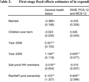
The estimations have been carried out using two-stage least squares within estimator. Table 2 shows the results for the first-stage logged per capita expenditure estimates for five health outcomes: general health status, subjective well-being, PCS-12, MCS-12, and HIV status. There are different first-stage estimates for the different health outcomes because the samples differ. Married, children ever born, and year variables are included because they are in the second stage, and they are excluded from the F-statistic tests of excluded instruments. Tables 3-7 show the results for the second-stage regressions.
4.1 First-stage regressions
Table 2 shows for the various health measures, the F-statistic of the excluded instruments in the first-stage regression of the IVs with all the other exogenous variables. For general health status, the F-statistic of 20.06 for the model with joint IVs is greater than 10 and significantly relevant (p<0.01). As expected, the coefficient for the interaction of salt price is negative and significant (-0.016); as the price of salt, a common household staple, increases, the individual and household available income decreases. The coefficient for the rainfall interaction is positive and significant (6.103);
10 Staiger and Stock (1997) formalized the definition of weak instruments. Many researchers conclude from
higher rainfall during the critical rainy season (otherwise very low) is associated with higher agricultural output (income).
The first-stage F-statistic for subjective well-being, PCS-12, and MCS-12 is 10.34, indicating that the model is unlikely to suffer from problems that arise with weak instruments, and it is acknowledged that the diagnostic is not as good as ideally would be the case. The coefficient for the salt price interaction is negative (-0.010) although not significant, and the rainfall interaction is positive and significant (9.945). The linear terms of the interactions are not included since they reduced the quality of the diagnostic tests. The differences observed in the first-stage regressions are due to the exclusion of the 2004 survey that did not assess these outcomes, whereas general health status and HIV status were assessed in all three waves (2004, 2006 and 2008). When the models for general health status and HIV status are restricted to two years of analysis (2006 and 2008), the first-stage results correspond to that of subjective well-being, PCS-12, and MCS-12 (results not shown).
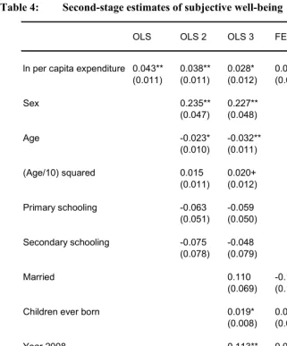
4.2 Second-stage regressions
Table 3 shows the second-stage estimates for general health status. There is a strong and highly-significant causal relationship between logged expenditure and general health status. For the IV-FE model, the coefficient for income is 0.409 and significant. For robustness checks, the Kleibergen-Paap Lagrange Multiplier test for underidentification is satisfied at 36.95 and significant. The Kleibergen-Paap Wald F-statistic for weak identification is 20.06, which falls at less than 10% of the maximal IV size of Stock-Yogo critical values.11 Lastly, Sargen-Hansen’s J-statistic of overidentification p-value is 0.064 and fails, but not by much, to reject the null hypothesis that the overidentifying restrictions are valid.12
11 Refer to Stock and Yogo (2005) for discussion on critical values based on Cragg-Donald statistic by Cragg
and Donald (1993). Weak instruments means having bias in the IV results >20% of the bias in first-stage results.
12 The overidentifying restriction means that the model is well-specified and the instruments are valid, i.e., do
Table 2: First-stage fixed effects estimates of ln expenditure
General health status
SWB, PCS-12,
and MCS-12 HIV result
Married -0.386+ -0.435 -0.349
(0.198) (0.309) (0.238)
Children ever born -0.023 0.026 -0.010
(0.030) (0.045) (0.031)
Year 2006 0.421** 0.437**
(0.102) (0.115)
Year 2008 1.146** 0.645** 1.195**
(0.119) (0.077) (0.134)
Salt price*HH members -0.016** -0.010 -0.016**
(0.004) (0.007) (0.005)
Rainfall*Land ownership 6.103** 9.945** 5.943**
(1.337) (2.596) (1.551)
Constant 5.849** 5.486** 5.726**
(0.284) (0.517) (0.321)
Adj R2
0.171 0.148 0.181
N 3540 2360 2790
F-statistic 20.06** 10.34** 14.81**
All the models presented support the rationale for using IV-FE and have been tested for the presence of endogeneity using the Durbin-Wu-Hausman test, which tests that under certain maintained assumptions the different estimators will yield similar point estimates. The tests are significant, demonstrating that the point estimates are different and the assumptions necessary for the different estimators to yield similar point estimates do not hold. That is, the endogenous regressor’s effect on the point estimates is meaningful, and instrumental variables techniques are required.
The interpretation of this model is: for a 10% increase in income there is a corresponding 0.039 increase in a categorical unit of general health status, or a 1.0% increase in mean health status. Interestingly, if the model is restricted to two years of analysis (2006 and 2008) for a minimum common overlap with other health outcomes, the effect of income is 0.826, which means a 10% increase in income is equal to a 0.079 unit increase in health status. The larger effect for the restricted sample can be explained by more and larger positive transitions in health status between the years 2006 and 2008, compared to those occurring between 2004 and 2008, or between 2004 and 2006 (0.037 unit increase for a 10% increase in income).
Table 3: Second-stage estimates of general health status
OLS OLS 2 OLS 3 FE IV-FE
ln per capita expenditure 0.031** 0.021** 0.020* 0.035** 0.409**
(0.008) (0.008) (0.008) (0.012) (0.096)
Sex 0.266** 0.275**
(0.037) (0.038)
Age -0.006 -0.013
(0.008) (0.009)
(Age/10) squared -0.005 0.0001
(0.010) (0.010)
Primary schooling 0.004 -0.025
(0.036) (0.037)
Secondary schooling 0.111 0.097
(0.069) (0.070)
Married 0.001 -0.066 0.094
(0.053) (0.078) (0.115)
Children ever born 0.011 0.005 0.021
(0.007) (0.013) (0.020)
Year 2006 0.204** 0.162** -0.077
(0.040) (0.039) (0.078)
Year 2008 0.063 -0.015 -0.569**
(0.039) (0.041) (0.151)
Constant 3.563** 3.839** 3.887** 3.518**
(0.049) (0.170) (0.187) (0.125)
N 3540 3540 3540 3540 3540
KP LM Underid 36.95**
KP Wald F-test 20.06**
Sargan p 0.064
Table 4: Second-stage estimates of subjective well-being
OLS OLS 2 OLS 3 FE IV-FE
ln per capita expenditure 0.043** 0.038** 0.028* 0.027 0.499**
(0.011) (0.011) (0.012) (0.017) (0.155)
Sex 0.235** 0.227**
(0.047) (0.048)
Age -0.023* -0.032**
(0.010) (0.011)
(Age/10) squared 0.015 0.020+
(0.011) (0.012)
Primary schooling -0.063 -0.059
(0.051) (0.050)
Secondary schooling -0.075 -0.048
(0.078) (0.079)
Married 0.110 -0.100 0.120
(0.069) (0.139) (0.213)
Children ever born 0.019* 0.033 0.032
(0.008) (0.022) (0.032)
Year 2008 0.113** 0.074+ -0.315*
(0.038) (0.041) (0.134)
Constant 3.739** 4.431** 4.440** 3.691**
(0.074) (0.214) (0.236) (0.212)
N 2360 2360 2360 2360 2360
KP LM Underid 17.69**
KP Wald F-test 10.34**
Sargan p 0.612
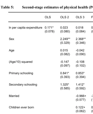
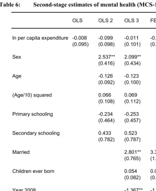
For SF-12 estimates in Tables 5 and 6, income does not have a significant result on either physical or mental health. While both coefficients are nonsignificant, both are of similar magnitude but have opposite signs; the physical health (PCS-12) coefficient is -0.575 and the mental health (MCS-12) is 0.525.
Table 5: Second-stage estimates of physical health (PCS-12)
OLS OLS 2 OLS 3 FE IV-FE
ln per capita expenditure 0.171* 0.023 0.018 0.061 -0.575
(0.078) (0.080) (0.084) (0.114) (0.683)
Sex 2.249** 2.368**
(0.329) (0.346)
Age 0.015 -0.042
(0.082) (0.090)
(Age/10) squared -0.147 -0.108
(0.097) (0.102)
Primary schooling 0.841* 0.853*
(0.393) (0.394)
Secondary schooling 1.325* 1.412*
(0.585) (0.592)
Married -0.966+ -3.287** -3.583**
(0.577) (1.111) (1.199)
Children ever born 0.122+ 0.166 0.167
(0.062) (0.131) (0.136)
Year 2008 -0.111 -0.463+ 0.062
(0.259) (0.278) (0.619)
Constant 51.36** 52.86** 54.63** 54.25**
(0.521) (1.757) (1.953) (1.484)
N 2360 2360 2360 2360 2360
KP LM Underid 17.69**
KP Wald F-test 10.34**
Sargan p 0.203
Table 6: Second-stage estimates of mental health (MCS-12)
OLS OLS 2 OLS 3 FE IV-FE
ln per capita expenditure -0.008 -0.099 -0.011 -0.099 0.525
(0.095) (0.098) (0.101) (0.144) (0.947)
Sex 2.537** 2.099**
(0.416) (0.434)
Age -0.126 -0.123
(0.092) (0.100)
(Age/10) squared 0.066 0.069
(0.108) (0.112)
Primary schooling -0.234 -0.253
(0.464) (0.457)
Secondary schooling 0.433 0.523
(0.782) (0.787)
Married 2.801** 3.311* 3.602*
(0.765) (1.547) (1.626)
Children ever born 0.054 0.030 0.029
(0.082) (0.189) (0.197)
Year 2008 -1.367** -1.394** -1.909*
(0.346) (0.382) (0.836)
Constant 54.86** 58.60** 55.80** 52.91**
(0.633) (1.941) (2.210) (2.001)
N 2360 2360 2360 2360 2360
KP LM Underid 17.69**
KP Wald F-test 10.34**
Sargan p 0.378
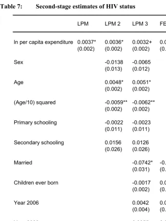
Table 7 shows the second stage results for HIV status where income has a 0.0055 coefficient; meaning a 10% increase in income results in a 0.052% higher probability of being tested HIV positive. Although not significant, this result corresponds to recent studies that show the disease predominantly affects the rich (Shelton et al. 2005; Mishra et al. 2007). The process through which income or wealth directly affects HIV status, however, is only poorly understood. Wealthier individuals tend to live in urban centers where HIV is more prevalent, they are more likely to be mobile, and they tend to have higher schooling which would appear to be protective of HIV risk. In this study, the direct relationship between income and HIV is largely unaffected by these issues because the sample analyzed is of the rural population that is poor and less mobile, therefore the estimates are conservative for extrapolations to urban areas at best.
The various second-stage OLS models including additional controls seem to affect the point estimates on the income variable very little for health, well-being, and HIV status (Tables 3, 4, 7 respectively). When comparing the coefficient changes of income from OLS to IV-FE, the prior might have been an overestimation in the OLS, but appears not to be the case for health and well-being in Tables 3 and 4, respectively. The magnitude of the point estimates on income is over twelve times as large in the IV-FE framework for both outcomes. That the IV-FE estimates are in fact much larger suggest attenuation bias due to measurement error in the OLS estimates rather than omitted variable bias or endogeneity, the latter two being perhaps quantitatively the most important issues for this study.13
13 One possible explanation for the divergence between OLS and IV-FE estimates is that the first stage
Table 7: Second-stage estimates of HIV status
LPM LPM 2 LPM 3 FE IV-FE
ln per capita expenditure 0.0037* 0.0036* 0.0032+ 0.0002 0.0055
(0.002) (0.002) (0.002) (0.001) (0.005)
Sex -0.0138 -0.0065
(0.013) (0.012)
Age 0.0048* 0.0051*
(0.002) (0.002)
(Age/10) squared -0.0059** -0.0062**
(0.002) (0.002)
Primary schooling -0.0022 -0.0023
(0.011) (0.011)
Secondary schooling 0.0156 0.0126
(0.026) (0.026)
Married -0.0742* -0.0120 -0.0099
(0.031) (0.010) (0.010)
Children ever born -0.0017 0.0009 0.0011
(0.002) (0.001) (0.001)
Year 2006 0.0042 0.0061* 0.0027
(0.004) (0.003) (0.004)
Year 2008 0.0055 0.0105** 0.0024
(0.006) (0.004) (0.007)
Constant 0.0164 -0.0657 0.0037 0.0374**
(0.010) (0.046) (0.053) (0.013)
N 2790 2790 2790 2790 2790
KP LM Underid 28.27**
KP Wald F-test 14.81**
Sargan p 0.332
5. Discussion
The analyses of the longitudinal MDICP/MLSFH data in this paper has permitted an advance in understanding how and to what magnitude income affects the health and well-being of individuals and families adjusting to and coping with AIDS-related health shocks and changing risk environments in rural Malawi. The estimates imply that a 10% increase in income raises mean general health status of rural Malawians by 1.0% and mean subjective well-being by 1.2%. An important point of distinction is that apart from HIV status, actual health outcomes are not measured in these analyses, but perceptions of health. The findings for the most part, therefore, are about how perceptions of health change with income. These are of interest even if they do not literally represent objective health measures because self-reported health is a widely-used measure of health status, has been validated in several studies, and there is a widely-reported consistent relationship between self-reported health and objective health outcomes.
An assumption in this study is that neither the interactions of salt price and the number of regular household members nor rainfall and land ownership determine directly an individual’s health—but only indirectly through income. Presumably, as the variation in rainfall is large and positive it drives up agricultural productivity and crop income. This in turn, affords families and individuals more income for health care and services, and also drives down prices of market goods. Similarly, the salt price alone does not directly determine health—salt is a commonly used daily staple and its price is correlated with income, which directly affects the income to health relationship. Concerns about the suitability of rainfall as an instrument, which can indirectly affect health by contributing to the growth of mosquito-born malaria where transmission is perennial with a peak following the January-April rainy season, might not alter the results. Since most adults have developed acquired-immunity to malaria illness, the groups at highest risk are children under five and pregnant women. However, children are not included in the sample, and there are few pregnant women in the sample, so their inclusion would not substantially affect the results.
The results indicate a positive causal relationship from income to health and well-being, lending support for current development programs of conditional cash transfers, income redistribution, resource allocation, income generation, and agricultural subsidies that could help in improving overall health and well-being in this population. Further studies can examine the relationship in controlled studies where these programs are currently in place. In this particular study, it may also be the case, however, that consumption expenditures are less applicable a measure of income than wage, non-wage, transitory income, or asset-based measures. In spite of this, consumption expenditures seem to be an appropriate and best-available measure for contemporaneous changes in the health outcomes analyzed in this context. If overall well-being and life-satisfaction of the population is the sole interest, then the data shows a slightly stronger causal pathway. There is potential for further studies of this causal relationship involving possibly better instruments, such as geographic access to markets or trading centers, which could have implications on isolating the influence of income on health. Even if a sizeable causal effect can be found, it does not preclude the command over many of the goods and services that promote health, such as better nutrition and access to safe water, sanitation, and quality health services that are severely lacking in rural Malawi and other contexts in Sub-Saharan Africa.
6. Acknowledgements
References
Acemoglu, D. and Johnson, S. (2007). Disease and development: The effect of life expectancy on economic growth. Journal of Political Economy 115(6): 925-985.
doi:10.1086/529000.
African Development Bank and OECD (2009). African Economic Outlook 2009. Paris: OECD.
Alderman, H., Behrman, J.R., Kohler, H.-P., Maluccio, J.A., and Watkins, S.C. (2001). Attrition in longitudinal household survey data. Demographic Research 5(4): 79-124. doi:10.4054/DemRes.2001.5.4.
Alderman, H., Hoddinott, J., and Kinsey, B. (2006). Long term consequences of early childhood malnutrition. Oxford Economic Papers 58(3): 450-474.
doi:10.1093/oep/gpl008.
Anglewicz, P., adams, j., Obare, F., Kohler, H.P., and Watkins, S.C. (2009). The Malawi Diffusion and Ideational Change Project 2004-06: Data collection, data quality, and analysis of attrition. Demographic Research 20(21): 503-540.
doi:10.4054/DemRes.2009.20.21.
Beegle, K. (2005). Labor effects of adult mortality in Tanzanian households. Economic Development and Cultural Change 53(3): 655-683. doi:10.1086/427410. Behrman, J.R. (2001). Why Micro Matters. In: Birdsall, N., Kelley, A.C., and Sinding,
S.W. (eds.). Population matters: Demographic change, economic growth, and poverty in the developing world. Oxford: Oxford University Press: 371-411. Behrman, J.R., Behrman, J.A., and Perez, N. (2009). On what diseases and health
conditions should new economic research on health and development focus? Health Economics 18(S1): S109-S128. doi:10.1002/hec.1464.
Behrman, J.R. and Knowles, J.C. (1999). Household income and child schooling in
Vietnam. World Bank Economic Review 13(2): 211-256.
doi:10.1093/wber/13.2.211.
Bignami-Van Assche, S., Reniers, G., and Weinreb, A.A. (2003). An assessment of the KDICP and MDICP data quality. Demographic Research S1(2): 31-76.
doi:10.4054/DemRes.2003.S1.2.
Change Project. Social Networks Project Working Papers; No. 6. Philadelphia: University of Pennsylvania.
Bignami-Van Assche, S., Van Assche, A., Anglewicz, P., Fleming, P., and Van De Ruit, C. (forthcoming). HIV/AIDS and time allocation in rural Malawi. Demographic Research.
Brückner, M. and Ciccone, A. (2007). Growth, democracy, and civil war. CEPR Discussion Paper 6568. London: Centre for Economic Policy Research.
Case, A. and Paxson, C. (2005). Sex differences in morbidity and mortality. Demography 42(2): 189-214. doi:10.1353/dem.2005.0011.
Case, A. and Wilson, F. (2000). Health and wellbeing in South Africa: Evidence from the Langeberg Survey. [unpublished report]. Princeton University.
Cragg, J.G. and Donald, S.G. (1993). Testing identifiability and specification in instrumental variables models. Econometric Theory 9(2): 222-240.
doi:10.1017/S0266466600007519.
Cutler, D., Deaton, A., and Lleras-Muney, A. (2006). The determinants of mortality. Journal of Economic Perspectives 20(3): 97-120. doi:10.1257/jep.20.3.97. Deaton, A. (2006). Global Patterns of Income and Health: Facts, Interpretations, and
Policies. WIDER Annual Lecture 10. Helsinki, Finland: UNU World Institute for Development Economics Research (UNU-WIDER).
Diener, E. (1994). Assessing subjective well-being: Progress and opportunities. Social Indicators Research 31(2): 103-157. doi:10.1007/BF01207052.
Diener, E. and Seligman, M.E.P. (2004). Beyond money: Toward an economy of well-being. Psychological Science in the Public Interest 5(1): 1-31.
doi:10.1111/j.0963-7214.2004.00501001.x.
Diener, E. and Suh, E.M. (1997). Measuring quality of life: Economic, social and subjective indicators. Social Indicators Research 40(1-2): 189-216.
doi:10.1023/A:1006859511756.
Dollar, D. (2001). Is globalization good for your health? Bulletin of the World Health Organization 79(9): 827-833. doi:10.1590/S0042-96862001000900007.
Easterlin, R.A. (2004). How beneficent is the market? A look at the modern history of mortality. In: Easterlin, R.A. (ed.). The Reluctant Economist. Cambridge: Cambridge University Press: 101-138.
Falaris, E.M. (2003). The effect of survey attrition in longitudinal surveys: Evidence from Peru, Côte d’Ivoire and Vietnam. Journal of Development Economics 70(1): 133-157. doi:10.1016/S0304-3878(02)00079-2.
Fenton, L. (2004). Preventing HIV/AIDS through poverty reduction: The only sustainable solution? Lancet 364(9440): 1186-1187. doi:10.1016/S0140-6736(04)17109-2.
Filmer, D. and Pritchett, L. (1999). The impact of public spending on health: Does money matter? Social Science & Medicine 49(10): 1309-1323.
doi:10.1016/S0277-9536(99)00150-1.
Filmer, D. and Pritchett, L. (2001). Estimating wealth effects without expenditure data--or tears: an application to educational enrollments in states of India. Demography 38(1): 115-132. doi:10.1353/dem.2001.0003.
Fitzgerald, J., Gottschalk, P., and Moffitt, R. (1998). The impact of attrition in the panel study of income dynamics on intergenerational analysis. Journal of Human Resources 33(2): 300-344. doi:10.2307/146434.
Fogel, R.W. (1997). New Findings on Secular Trends in Nutrition and Mortality: Some Implications for Population Theory. In: Rosenzweig, M. and Stark, O. (eds.). Handbook of Population and Family Economics. Amsterdam: Elsevier: 433-481. Fogel, R.W. (2004). The Escape from Hunger and Premature Death, 1700-2100.
Cambridge and New York: Cambridge University Press.
Fordyce, M.W. (1988). A review of research on the happiness measure: A sixty second index of happiness and mental health. Social Indicators Research 20(4): 355-381. doi:10.1007/BF00302333.
Fortson, J.G. (2008). The gradient in Sub-Saharan Africa: Socioeconomic status and HIV/AIDS. Demography 45(2): 303-322. doi:10.1353/dem.0.0006.
Gillespie, S., Kadiyala, S., and Greener, R. (2007). Is poverty or wealth driving HIV transmission? AIDS 21(S7): S5-S16. doi:10.1097/01.aids.0000300531.74730.72. Guha, S. (1994). The importance of social intervention in England’s mortality decline:
The evidence reviewed. Social History of Medicine 7(1): 89-113.
Halperin, D.T. and Allen, A. (2000). Is poverty the root cause of African AIDS? AIDS Analysis Africa 11(4): 1-15.
Hoddinott, J., Maluccio, J.A., Behrman, J.R., Flores, R., and Martorell, R. (2008). Effect of a nutrition intervention during early childhood on economic
productivity in Guatemalan adults. Lancet 371(9610): 411-416.
doi:10.1016/S0140-6736(08)60205-6.
Huffman, G.J., Adler, R.F., Bolvin, D.T., Gu, G., Nelkin, E.J., Bowman, K.P., Hong, Y., Stocker, E.F., and Wolff, D.B. (2007). The TRMM multi-satellite precipitation analysis: Quasi-global, multi-year, combined-sensor precipitation estimates at fine scale. Journal of Hydrometeorology 8(1): 38-55.
doi:10.1175/JHM560.1.
Kohler, H.-P., Behrman, J.R., and Watkins, S.C. (2007). Social networks and
HIV/AIDS risk perceptions. Demography 44(1): 1-33.
doi:10.1353/dem.2007.0006.
Lanjouw, P. and Ravallion, M. (1995). Poverty and household size. Economic Journal 105(433): 1415-1434. doi:10.2307/2235108.
McKeown, T. (1979). The Role of Medicine: Dream, Mirage, or Nemesis? Princeton, NJ: Princeton University Press.
Miguel, E., Satyanath, S., and Sergenti, E. (2004). Economic shocks and civil conflict: An instrumental variables approach data set. Journal of Political Economy 112(4): 725-753. doi:10.1086/421174.
Mishra, V., Bignami-Van Assche, S., Greener, R., Vaessen, M., Hong, R., Ghys, P.D., Boerma, J.T., Van Assche, A., Khan, S., and Rutstein, S. (2007). HIV infection does not disproportionately affect the poorer in sub-Saharan Africa. AIDS 21(S7): S17-S28. doi:10.1097/01.aids.0000300532.51860.2a.
National Statistical Office (NSO) [Malawi], and ORC Macro. (2005). Malawi Demographic and Health Survey 2004. Calverton, Maryland: NSO and ORC Macro
National Statistical Office of Malawi (2010). Rural Price Indices [data file]. Zomba, Malawi: National Statistical Office of Malawi.
Pavot, W. and Diener, E. (1993). Review of the satisfaction with life scale. Psychological Assessment 5(2): 164-172. doi:10.1037/1040-3590.5.2.164. Paxson, C.H. (1992). Using weather variability to estimate the response of savings to
transitory income in Thailand. American Economic Review 82(1): 15-33.
Preston, S.H. (1975). The changing relation between mortality and level of economic development. Population Studies 29(2): 231-248. doi:10.2307/2173509.
Preston, S.H. (1980). Causes and consequences of mortality declines in less developed countries during the twentieth century. In: Easterlin, R.A. (ed.). Population and Economic Change in Developing Countries. Chicago, IL: University of Chicago Press for National Bureau of Economic Research: 289-360.
Preston, S.H. (1996). American longevity, past, present, and future. Policy Brief No. 7/1996. Syracuse, NY: Maxwell School Center for Policy Research.
Pritchett, L. and Summers, L.H. (1996). Wealthier is healthier. Journal of Human Resources 31(4): 841-868. doi:10.2307/146149.
Shelton, J.D., Cassell, M.M., and Adetunji, J. (2005). Is poverty or wealth at the root of HIV? Lancet 366(9491): 1057-1058. doi:10.1016/S0140-6736(05)67401-6. Staiger, D. and Stock, J.H. (1997). Instrumental variables regressions with weak
instruments. Econometrica 65(3): 557-586. doi:10.2307/2171753.
Steckel, R.H. (1995). Stature and the standard of living. Journal of Economic Literature 33(4): 1903-1940.
Stock, J.H. and Yogo, M. (2005). Testing for weak instruments in linear IV regression. In: Andrews, D.W.K. and Stock, J.H. (eds.). Identification and Inference for Econometric Models: Essays in Honor of Thomas Rothenberg. Cambridge: Cambridge University Press: 80-108.
Strauss, J. and Thomas, D. (1998). Health, nutrition and economic development. Journal of Economic Literature 36(2): 766-817.
Szreter, S. (1988). The importance of social intervention in Britain’s mortality decline c. 1850-1914: A reinterpretation of the role of public health. Social History of Medicine 1(1): 1-37. doi:10.1093/shm/1.1.1.
Thomas, D. and Strauss, J. (1992). Prices, infrastructure, household characteristics, and child height. Journal of Development Economics 39(2): 301-331.
Thomas, D. and Strauss, J. (1997). Health and wages: Evidence on men and women in urban Brazil. Journal of Econometrics 77(1): 159-185. doi:10.1016/S0304-4076(96)01811-8.
Thomas, D., Strauss, J., and Henriques, M. (1990). Child survival, height for age, and household characteristics in Brazil. Journal of Development Economics 33(2): 197-234. doi:10.1016/0304-3878(90)90022-4.
Üstün, T.B., Ayuso-Mateos, J.L., Chatterji, S., Mathers, C., and Murray, C.J.L. (2004). Global burden of depressive disorders in the year 2000. The British Journal of Psychiatry 184(5): 386-392. doi:10.1192/bjp.184.5.386.
Vyas, S. and Kumaranayake, L. (2006). Constructing socio-economic status indices: How to use principal components analysis. Health Policy and Planning 21(6): 459-468. doi:10.1093/heapol/czl029.
Ware, J.E., Kosinksi, M., and Keller, S.D. (2001). SF-12: How to Score the SF12 Physical & Mental Health Summary Scales, Third Edition. Lincoln, RI: QualityMetric.
Ware, J.E., Kosinski, M., and Keller, S.D. (1996). A 12-item short-form health survey: Construction of scales and preliminary tests of reliability and validity. Medical Care 34(3): 220-233. doi:10.1097/00005650-199603000-00003.
Watkins, S.C., Behrman, J.R., Zulu, E.M., and Kohler, H.-P. (2003). Introduction to “Research on demographic aspects of HIV/AIDS in rural Africa”. Demographic Research S1(1): 1-30. doi:10.4054/DemRes.2003.S1.1.
Wolpin, K.I. (1982). A new test of the permanent income hypothesis: The impact of weather on the income and consumption of farm households in India. International Economic Review 23(3): 583-594. doi:10.2307/2526376.
World Bank (2002). Globalization, Growth, and Poverty: Building an Inclusive World Economy. Oxford and Washington, DC: Oxford University Press and The World Bank.
World Bank (2007). Malawi - Poverty and vulnerability assessment: Investing in our future. World Bank Poverty Assessment; Report No. 36546-MW. Washington, DC: World Bank.
Appendix
Figure A-1: Monthly accumulated rainfall