Volume 25 - Article 23 | Pages 723–754

(1)

Max Planck Institute for Demographic Research Konrad-Zuse Str. 1, D-18057 Rostock·GERMANY www.demographic-research.org

DEMOGRAPHIC RESEARCH

VOLUME 25, ARTICLE 23, PAGES 723-754

PUBLISHED 15 NOVEMBER 2011

http://www.demographic-research.org/Volumes/Vol25/23/ DOI: 10.4054/DemRes.2011.25.23

Research Article

Constraint or choice? Disentangling fertility

determinants by switching regressions

Christoph Sax

c

°2011 Christoph Sax.

(2)

2 Conceptual framework 726

2.1 A constrained optimization framework 727

2.2 Factors influencing the demand for children 728 2.3 Factors influencing the Malthusian constraint 729

2.4 The problem of birth control 730

2.5 The problem of aggregation 730

3 Estimation by switching regressions 731

3.1 The model 731

3.2 Derivation of the likelihood function 733

3.3 Specification 735

4 Data 735

5 Results 740

5.1 The basic model 740

5.2 Specific explanatory variables 743

6 Conclusion 746

7 Acknowledgements 748

References 749

A Appendix 752

A.1 An expression for the assignment probability 752

(3)

Constraint or choice?

Disentangling fertility determinants by switching regressions

Christoph Sax1

Abstract

In 1953, many poor countries had not yet approached the demographic transition. Ac-cordingly, income generally had a positive impact on fertility in poor countries, while it has a negative impact today. Easterlin’s supply-demand framework offers an explanation for this nonlinearity by attributing the positive relationship to Malthusian (or “supply”) factors and the negative relationship to “demand” factors.

This paper estimates Easterlin’s supply-demand framework by switching regressions in a panel data set of 152 countries from 1953 to 1998. The technique allows the identifi-cation of several factors affecting the Malthusian constraint and the demand for children, such as income, source of income, urbanization, religion and medical environment.

It is found that a combination of higher GDP per capita, a decrease in infant death rate and an increase in education explain a substantial part of the reversal of the relationship between income and net fertility over the sample period.

1_{University of Basel, Department of Business and Economics, Jakob Burckhardt Haus, 4001 Basel,}

(4)

1. Introduction

A striking fact in human population history is the reversal of the relationship between income and fertility. In order to reveal the causes of the reversal, this paper estimates Easterlin’s supply-demand framework by switching regressions in a panel data set of 152 countries from 1953 to 1998.

Until late in the 19th century, richer individuals tended to have more children than did poorer individuals (Stys 1957; Schapiro 1982; Weir 1995; Lee 1987); today, richer individuals tend to have fewer (Docquier 2004). A similar reversal of the relationship can be observed in cross-country data. As it has been put by Thomas Malthus in 1798 (Malthus 1986): “The reason that the greater part of Europe is more populous now than it was in former times, is, that the industry of the inhabitants has made these countries produce a greater quantity of human subsistence.” These days the opposite is true. Around the world, richer countries tend to have a lower birth rate and therefore a lower (and sometimes negative) population growth rate.

There are two sets of explanations for these empirical findings: Malthusian expla-nations are commonly used to characterize a positive relationship between income and fertility. According to Malthus, “preventive” as well as “positive checks” force poor peo-ple to have fewer children. Thereby, the fear of material difficulties acts as a preventive check. It causes people to moderate their sexual desires, to contracept or to delay mar-riage. If ineffective, the more ferocious “positive checks” will come into force. Diseases and famine increase the mortality rates of poor people in particular and reduce their re-production rates.

On the other hand, modern fertility theory focuses on the demand for children and explains why there is a negative relationship between income and fertility. It suggests several factors leading to a negative correlation between these two variables: increased investment in education or the “quality” of children (Becker and Lewis 1973; Becker and Tomes 1976), higher relative wages of women (Galor and Weil 1996, 1999) or a reduction in the contribution made by children to family income (Caldwell 1976).

(5)

The main contribution of this paper is the use of switching regressions in order to si-multaneously estimate the Malthusian constraint and the demand for children as compo-nents of net fertility. In a simplified form, Easterlin’s supply-demand framework exactly corresponds to an econometric switching regression model, in which the observed value of the dependent variable is the minimum of two latent variables.

This paper presents a simplified version of Easterlin’s supply-demand framework, which is used as the conceptual underpinning of the empirical model. Unlike Montgomery (1987), who presented an application of the switching regression methodology to the World Fertility Survey data, this paper uses cross country panel data from 152 countries from 1953 to 1998.2

In 1953, many poor countries had not yet completed the demographic transition. Ac-cordingly, Malthusian factors dominated demand factors in these countries, resulting in a positive relationship between income and net fertility in poor countries. In 1998, with almost all countries having completed their demographic transition, net fertility is deter-mined by demand factors everywhere, resulting in a negative relationship between income and net fertility.

Switching regressions may help to answer several important questions: Why was there a positive relationship for low-income countries in 1953, and why has it changed into a negative one? Can we explain these changes in terms of shifts in the Malthusian constraint and in demand? What other factors, beside income, determine the Malthusian constraint and the demand for children?

The switching regression technique makes it possible to elegantly deal with the non-linearity of the relationship between income and net fertility: First of all, switching re-gressions are based on theory. The two underlying components have a theoretical inter-pretation in line with Easterlin’s supply-demand framework. The positive branch of the relationship between income and net fertility can be interpreted as the result of Malthusian mechanisms, while the negative branch is the result of demand effects. Second, shifts in these underlying components may be quantified. Over time, there is not only a reversal of the relationship between income and net fertility; there is also a systematic upward shift of the positive branch of the relationship and a downward shift of the negative branch. Third, thanks to its parametric structure, multiple explanatory variables may be analyzed in a switching regression model, including fixed effects in panel data, and statistical in-ference tests may be carried out. Depending on whether a variable affects demand or

2_{While Montgomery’s work is similar to this article in the application of the switching regression}

(6)

the Malthusian constraint, its impact on fertility may be different. Switching regressions allows one to distinguish between the effects on demand and the Malthusian constraint. Finally, on a technical level, there is no need to know whether an observation was caused by the Malthusian constraint or by the demand for children. Instead, the switching regres-sion method used in this paper allows for the calculation of assignments probabilities; i.e., values representing the probability of belonging either to the constraint or to the demand. Conceptually, this paper borrows mainly from Easterlin’s supply-demand framework. It has reduced Easterlin’s three components of fertility to two components, and represents them in an unified optimization framework along the lines of Galor and Weil (1999). The main focus of this paper is empirical. While several determinants of the Malthusian constraint and demand are briefly discussed from a theoretical point of view in the next section, the focal point of the paper is the estimation of their impact using switching regressions.

The estimation of the switching regression framework reveals the following: Malthu-sian factors, while important in 1953, weakened over time and have lost their significance today; demand factors, on the other hand, have become more important. This shift from the Malthusian constraint to the demand for children is sufficient to explain the reversal of the relationship between income and the number of surviving children over the sample period.

This paper is organized as follows: Section 2. discusses the conceptual framework in more detail. Section 3. outlines the adaption of a switching regression model to the setting. Section 4. covers the data. Section 5. presents the results of the estimations.

2. Conceptual framework

(7)

2.1 A constrained optimization framework

The utility that parents get from their children depends on both the quantity and the quality of the children and is represented by:

U =f(c, n, q) (1)

wherecis the parents’ consumption,nis the number of surviving children andqis the quality of children, which is assumed to be identical for all children. “Quality” has the same meaning as in Becker (1960, p. 211); it is the result of nursing, education and other investments of time or money. The analysis focuses on the number of surviving children, as parents are primarily interested in children growing into adulthood.

Parents spend their income on children and consumption goods, according to the fol-lowing budget constraint:

nqp+c=I (2)

wherepis the price for a quality-unit of a child andIis total income. Prices are denoted in terms of consumption goods, the price of one unit ofc is therefore equal to 1. The unit-price (or “shadow”-price) of a child is proportional to the level of quality. Similarly, the price of a unit of quality for each child is proportional to the number of children. Consequently, as long as the income elasticity of quantity is sufficiently smaller than the income elasticity of quality, a negative relationship between income and the number of children occurs (see Becker and Lewis (1973) for a more lengthy discussion on the subject).

The solution to the optimization problem can be written the following way:

nD=f(I, p) (3)

nDis the interior solution to the maximization problem and will be defined as thedemand for children. Note that, given the assumption on the income elasticities of quantity and quality, the relationship betweenIandnDis negative.

While Eq. (3) appropriately describes the optimal fertility decisions for high levels of income, it does not for very low levels. If parents are poor, they cannot lower their consumption to arbitrary low levels, nor can they lower their children’s consumption. There is a minimal consumption constraint for the parents as well as a minimal quality requirement for a child:

c ≥ cmin (4)

(8)

In order to keep the discussion simple, it is assumed that these constraints are binding at the same level of income, thereby excluding a situation where only one constraint is binding. If both constraints are binding, the budget constraint (2) can be rewritten:

nC =I−cmin

qminp (6)

Socmin,qminandIare constraining the possible number of surviving children. The op-timization problem now becomes trivial as parents choose the maximum possible number of surviving children. Therefore,nC, defined as theMalthusian constraint, is a bound-ary solution to the maximization problem in (1) and (2), when the minimal consumption constraint and the minimal quality requirement are binding. Note that the relationship betweenIandnCis positive.

Above a certain level of income,nA, the overall solution to the maximization problem, is equal tonD; below,nAis equal tonC. Equivalently, the solution can be represented in the following form:

nA= min(nD, nC) (7)

which states that the actual number of surviving children is the minimum of the demand for children and the Malthusian constraint. Note that the relationship betweenIandnA is increasing first and then decreasing, showing the empirically observed hump-shaped pattern.

2.2 Factors influencing the demand for children

In Eq. (3), the negative relationship betweenIandnDarises from the substitution of child quantity by child quality, which is itself the result of different income elasticities of quan-tity and quality, as has been argued by Becker and Lewis (1973). However, the negative relationship may be reinforced by alternate mechanisms. For instance, if childrearing is done predominantly by women, higher relative wages for women will increase the oppor-tunity costs of having children and thus reduce demand for them (Galor and Weil 1996, 1999).

(9)

income (Caldwell 1976). Therefore, even if Becker’s assumption about the income elas-ticities of quantity and quality is not valid, the relationship betweenIandnDin Eq. (3) may still be negative.

The strength of the negative relationship betweenIandnDalso depends on the source ofI. If an increase inIis the result of an increase in the wage, we would expect a strong negative relationship, due to the increased opportunity costs of childrearing. On the other hand, ifIrepresents a pure increase in income without an effect on opportunity costs (e.g., by selling oil), a less pronounced relationship has to be expected. Finally, the demand for children may depend on religion or culture. If cultural acceptance of small families becomes more popular, individual preferences will be shifted towards a lower number of children (McQuillan 2004; Fernandez and Fogli 2006).

2.3 Factors influencing the Malthusian constraint

As is obvious from Eq. (6), income relaxes the Malthusian constraint, by making more surviving children affordable. Other than income, improvements in general health condi-tions will lead to an increase in the Malthusian constraint: In Eq. (6), an improvement in general health conditions can be thought of as a reduction inqmin, the minimal quality requirement for a child. Most obviously, a reduction in child mortality leads to a lower qminby lowering the number of births necessary to achieve a certain number of surviving children. Also, birth costs may be reduced as the number of miscarriages decreases and the risk for a mother during pregnancy falls. Finally, minimal child care costs may be reduced, as, for example, an improvement in sanitation makes breastfeeding less indis-pensable.

(10)

2.4 The problem of birth control

Up to this point, it has been assumed that people are always able to control their fertility. If that is not the case, actual fertility will be higher than the minimum of demand and the constraint. As long as the Malthusian constraint is binding, contraception failure will not increase the number of surviving children, as Malthusian “positive checks” will make up for the failure. A failure of birth control could even reduce the number of surviving children.

However, as soon as the demand for children determines the actual number of surviv-ing children, excess fertility could occur. The magnitude of excess fertility depends on income in two opposite ways. First, an increase in income widens the potential fertility regulation gapnC−nD. Second, it eases the access to contraceptions. For high levels of income, the second effect will eventually dominate.

In the following, the problem of birth control will not be pursued further, as it is diffi-cult to incorporate it into the switching regression setting. Furthermore, the omission may be justified by the analysis of Pritchett (1994), who finds that, a) on an aggregate level, there is a very close relationship between desired and actual fertility; b) the costs and availability of contraceptives have no effect on desired fertility; and c) the costs and avail-ability of contraceptives have only a very small effect on excess fertility. He concludes, that, while contraceptive prevalence is an important proximate determinant of fertility, it is negligible as an ultimate causal determinant of fertility. Contraceptive use is higher in countries with lower fertility because desired fertility is lower in these countries.

2.5 The problem of aggregation

Aggregating Eq. (7) leads to another complication: On an aggregate level, the minimal condition would be only valid if all individuals in a country were equal and were repre-sented by a ‘representative agent’. If individuals differ of their characteristics, the average value ofnAis systematically lower than the minimum of the averages ofnDandnC:

¯

nA= 1

n N

X

i=1

min(nDi, nCi)≤min(¯nD,¯nC)

For example, a rich and a poor couple may have the same low value of nA for very different reasons: The rich couple’s fertility is determined bynD, while the poor couple’s fertility is determined bynC. Thus, in theory, the higher the income inequality, the more pronounced is the downward bias.

(11)

(1984) and Drèze and Bean (1988). It can be shown analytically that, under the assump-tion of a log-normal distribuassump-tion, the aggregaassump-tion leads to an expression of a ‘Constant Elasticity of Substitution’ (CES) form, which smooths the relationship.

There are two reasons that the problem is of minor importance in practice: First, in a Monte Carlo analysis, Quandt (1986) has shown that, from an econometric perspective, the individual model, applied to aggregate data, often leads to better estimations than the aggregated CES model. Second, in our specification, the inclusion of Gini-coefficients will shift the demand for children and the constraint in opposite directions (it decreases the Malthusian constraint and it increases demand, possibly acting as a proxy for some other development-related factors; see specification (9) in the appendix). If the downward bias was severe, both functions would be affected negatively.

In the following,nA,¯ ¯nD, andnC¯ are used in the same way as the individual functions, and the notation of averages will be ignored from here on.

3. Estimation by switching regressions

3.1 The model

Let us start with a linear formulation of the framework from the previous section:

nDi = x0DiβD+uDi (8)

nCi = x0

CiβC+uCi (9)

nAi = min(nCi, nDi) (10)

The first two equations are restatements of the demand for children (3) and the Malthusian constraint (6). BothnDiandnCiare combinations of independent variables,xDiandxCi, which both may include the same variables; and an equation-specific error term,uDior uCi. The third equation is identical to the minimum condition (7) and links the demand for children and the Malthusian constraint to the actual number of surviving children.

BothnDiandnCiare latent variables. For each unit, at any point in time, there is a realization of both the demand for children and the Malthusian constraint. However, only the lower of the two is relevant fornAi. Because data is available only onnAi, being the lower one ofnDi, andnCiis the only way for a latent variable to become observable.

(12)

supply, however, the supplied quantity is traded – there are people without homes. As long as there is no data on supply and demand, these underlying functions need to be estimated from data on the number of houses actually traded.

In the present setting,nCiis observable as long as it is lower thannDi. Economically, this implies that consumption and child quality are equal to their lower bounds, and there-fore the actual number of surviving children is determined by the budget constraint. Such a situation is more likely, for example, if the country has a bad medical environment (a lownCi) and a high prevalence of child labor (a highnDi). Similarly, it is more likely for net fertility to be determined bynCiif a country is poor, as being poor implies both a low nCiand a highnDiat the same time.

How is such a model to be estimated? As mentioned, no information aboutnCiornDi is available, nor about whether an observation ofnAiwas actually determined bynCior nDi. If the second item of information were available, one could imagine estimating (8) and (9) by OLS. This is, by the way, what Fair and Jaffee did. However, this approach would lead to misleading results. The problem is that whether a value ofnCi is lower thannDior not depends not only onnCi, but also onnDi. Thus, both equations need to be estimated simultaneously.

(13)

3.2 Derivation of the likelihood function

In order to derive the likelihood function of this model, it will be assumed thatuDiand uCiare independent (σ2

D,C = 0),3 serially uncorrelated and normally distributed with a mean of zero and a variance ofσ2

DandσC2, respectively. Using Eq. (8) and (9) and the assumptions about the distribution of the error terms, the distribution and the density functions can be written down.4

Let us consider the case in which actual fertility is determined by the Malthusian constraint; i.e.,nAi=nCi. In this case, the conditional density function ofnAiis given by:

h(nAi|nCi< nDi) = Z _∞

nAi

g(nAi, nDi)dnDi/Πi (11)

= fC(nAi)(1−FD(nAi))/Πi

g(nDi, nCi)denotes the joint density function ofnDiandnCi. BecauseuDianduCiare independent,g(nDi, nCi)is equal tofD(nDi)·fC(nCi). Additionally,Πi is defined as the probability that an observation of actual net fertility is determined by the Malthusian constraint (Πi ≡ Pr(nCi < nDi)). Intuitively, the integral denotes the likelihood of nAi =nCitimes the probability thatnDi > nAi. Dividing the integral byΠiyields the likelihood ofnAi, given thatnAi=nCi.

3_{There are variables (e.g. income) that affect both the Malthusian constraint and the demand for children.}

If such a variable was omitted, the errors would be correlated. The assumption of independence thus requires that the model is correctly specified and no major factor affecting both functions has been omitted. Goldfeld and Quandt (1978) have extended the present method to positive or negative correlations between the residuals. However, their method frequently leads to nonsensical results – as in the present case, where the correlation converges towards +1.

4_{Solving (8) and (9) for the error term and substituting into the normal density and distribution function, one}

gets:

fD(nDi) = √ 1 2πσDexp

"

− 1 2σ2

D

(nDi−β0DxDi)2

#

fC(nCi) = √ 1 2πσC exp

"

− 1 2σ2

C

(nCi−βC0 xCi)2

#

FD(nDi) =

ZnDi

−∞ fD(nDi)dnDi= Φ µ

nDi−β0

DxDi σD

¶

FC(nCi) =

ZnCi

−∞

fC(nCi)dnCi= Φ

µ

nCi−β0

CxCi σC

(14)

On the other hand, ifnAi = nDi, the conditional density function ofnAi may be derived along the same lines:

h(nAi|nCi> nDi) = fD(nAi)(1−FC(nAi))/(1−Πi)

AsnAiis determined bynCiwith probabilityΠiand bynDiwith probability1−Πi, the unconditional density function ofnAiis the weighted sum of the conditional density functions (11) and (12):

h(nAi) = Πih(nAi|nCi< nDi) + (1−Πi)h(nAi|nCi> nDi)

= fC(nAi)(1−FD(nAi)) +fD(nAi)(1−FC(nAi))

Intuitively, (12) denotes the likelihood of an observation of actual net fertility, given that it is determined either by the Malthusian constraint or the demand for children, and given the fact that the lower component of the two determines actual fertility. Hence, the likelihood function is the product of (12) for allNobservations:

L =

N

Y

i=1

h(nAi) (12)

In order to estimate the model, the parametersβD,βC,σ2

DandσC2 have to be chosen such that the value of (12) is maximized.5

Ex-post, with the estimations of the parameter in hand, the probability that an obser-vation of actual fertility is determined by the demand for children (APi = Pr(nCi < nDi|nAi))or by the Malthusian constraint (1−APi) can be calculated (See the appendix for the derivation ofAPi). Thus, estimating the model will also reveal information that was missing in the beginning; i.e., it will tell us whether a country’s net fertility was determined by the Malthusian constraint or by the demand for children.

5_{In order to maximize (12), the coefficients}_βD_and_βC _{must be chosen numerically. In the present case,}

maximization is not without problems: First, the likelihood function is unbounded for certain parameter values. If, for example,σ2

(15)

3.3 Specification

The simplest specification of a switching regression model contains the net rate of re-production (NRR) as its left-hand variable, and one single exogenous variable, GDP per capita, included both in thenCiand in thenDifunction. This most parsimonious spec-ification is not fully identified, as both functions are based on the same set of variables. Thus,nCican be arbitrarily interchanged withnDi. Contrary to what one expects from a traditional equilibrium model, such an unidentified model may be estimated nevertheless. In order to reach identification, some additional identifying assumption has to be made. For example, it may be assumed that demand has a negative slope in GDP per capita, while the constraint has a positive slope. This is indeed what we do as a starting point in Section 5.

Full identification is reached by including additional, function-specific variables. While GDP per capita is generally included in both functions, several demand-specific variables will be used as well. We will include measures on religion, education, urbanization and oil exports in order to analyze their specific effect on the demand for children. As for supply-specific variables, a child mortality measure will be used as a proxy for the gen-eral medical environment. Finally, the use of a time trend variable allows for tracing the nCiandnDifunction over time. Alternatively, time dummy variables may be included in order to control for any time-specific effects on both functions.

4. Data

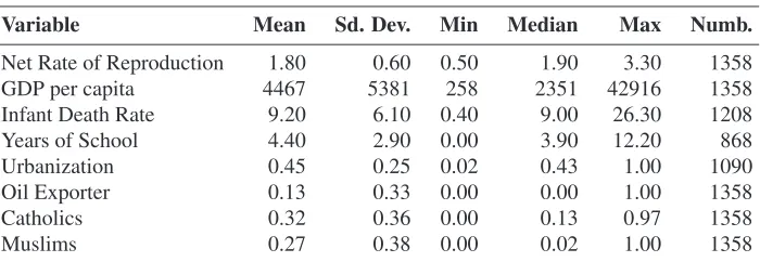
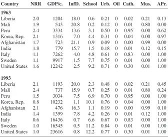
This section deals with the choice of the data. Table 1 shows the descriptive statistics of the variables in use, while Table 2 offers some examples for several countries in different world regions and time periods.

There are at least three ways to measure fertility: population growth rates, total fertil-ity or net reproduction rates. While population growth rates are problematic, as they are influenced by immigration and age structure, total fertility rates do not account for child mortality. That leaves us with net reproduction rates (NRR). The NRR is the hypothetical number of surviving girls a woman could give birth to in her lifetime. It is calculated as the sum of all age-specific fertility rates times the probability of reaching the correspond-ing age.6 _{Because the NRR covers only girls, the actual number of surviving children}

6_{Formally, the NRR may be written as:}

NRR =

7

X

i=1

ASFRd i ·SRdi

where ASFRd

1is the age-specific probability of women between 15 and 19 giving birth to a daughter; ASFRd2is the age-specific probability of women between 20 and 24 giving birth to a daughter, etc. ASFRd

(16)

is approximately twice as high. A useful trick is to think of NRR numbers as pairs of children. Data on NRR has been taken from the Demographic Yearbook of the United Nations (United Nations Statistics Division 2001). The source contains an NRR num-ber for every fifth year between 1953 and 1998, a maximum of 10 observations for each country. Altogether, data for 152 countries is available, but as some values are missing, the total number of observations is 1358.

GDP per capita is used as a proxy for income, as it is estimated by Maddison (2003). The values are noted in purchasing power adjusted dollars of 1990. It is thus possible to compare those numbers between countries and over time. In fitting the data to the assumption of a normal distribution, logs are taken of all values of GDP. However, in Tables 1 and 2, non-logarithmic values are reported.

Table 1: Descriptive statistics — Net rate of reproduction, GDP per capita (PPP Dollars of 1990), infant death rate (%), education (years), ur-banization (fraction), heavily dependent on oil (dummy), Catholics (fraction), Muslims (fraction)

Variable Mean Sd. Dev. Min Median Max Numb.

Net Rate of Reproduction 1.80 0.60 0.50 1.90 3.30 1358

GDP per capita 4467 5381 258 2351 42916 1358

Infant Death Rate 9.20 6.10 0.40 9.00 26.30 1208 Years of School 4.40 2.90 0.00 3.90 12.20 868

Urbanization 0.45 0.25 0.02 0.43 1.00 1090

Oil Exporter 0.13 0.33 0.00 0.00 1.00 1358

Catholics 0.32 0.36 0.00 0.13 0.97 1358

Muslims 0.27 0.38 0.00 0.02 1.00 1358

the age-specific probability of women between 45 and 49 giving birth to a daughter. SRd

i is the probability that a daughter reaches the age of the mother. In this version of the NRR as well as in the in the Demographic Yearbook, ASFRd

(17)

Table 2: Examples, 1963 and 1993 — Net rate of reproduction, GDP per capita (PPP Dollars of 1990), infant death rate (%), education (years), urbanization (fraction), heavily dependent on oil (dummy), Catholics (fraction), Muslims (fraction), Assignment probability (based on specification (6) from Table 4)

Country NRR GDP/c. InfD. School Urb. Oil Cath. Mus. APr. 1963

Liberia 2.0 1204 18.0 0.6 0.21 0 0.02 0.21 0.13 Mali 1.9 543 20.8 0.2 0.12 0 0.01 0.80 0.00 Peru 2.4 3334 13.6 3.1 0.50 0 0.95 0.00 0.62 Korea, Rep. 2.1 1316 7.0 4.4 0.31 0 0.04 0.00 0.97 Afghanistan 1.7 723 21.1 0.9 0.09 0 0.00 0.99 0.00 India 1.8 779 15.7 1.5 0.18 0 0.01 0.12 0.15 Italy 1.1 7262 4.0 4.8 0.61 0 0.83 0.00 1.00 Sweden 1.1 9917 1.5 7.7 0.75 0 0.01 0.00 1.00 United States 1.6 12242 2.5 9.2 0.71 0 0.30 0.01 1.00

1993

(18)

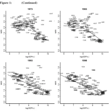
Figure 1 plots the evolution of the relationship between logarithmic GDP per capita and the NRR in the sample data. The line represents a nonparametric estimation of the relationship.7 _{The simple bivariate plots already reveal a striking reversal of the} relation-ship between income and net fertility. While there was a positive relationrelation-ship for poor countries in 1953, the relationship is negative for all levels of income in 1998.

Several additional variables are used for the estimation of the demand for children and the Malthusian constraint. The infant death rate, taken from the Demographic Yearbook (United Nations Statistics Division 2001), serves as a proxy for the medical environ-ment. Schooling data has been taken from the Barro-Lee data set on educational attain-ment (Barro and Lee 2000). The percentage value of urbanized households, the number of physicians per 1000 and Gini-coefficients are from the World Developing Indicators database (World Bank 2008). The percentage values of Catholics and Muslims are taken from a data set of a paper by La Porta et al. (1999). Finally, a dummy variable indicates whether a country is heavily dependent on oil or not. If the earnings of oil exports ex-ceed 10% of GDP, a country is defined as heavily dependent on oil. The data about oil dependency are from Ross (2001); the United Arab Emirates were added by the author.

Figure 1: Net reproduction rate (NRR) and logarithmic GDP per capita for

six points in time between 1953 and 1998; the line denotes a

non-parametricLOESSestimation withα= 0.8

7_{The method in use is a local regression with a variable bandwidth known as}_LOESS_{. A tricubic kernel and a}

(19)

(20)

5. Results

5.1 The basic model

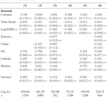
The first specification contains the NRR as its left-hand variable, and GDP per capita as the only exogenous variable included in both functions. Each point in time from 1953 to 1998 is examined separately. The results of these estimations for three points in time are reported in Table 3. In line with expectations, the GDP per capita coefficient in the constraint function is positive, while it is negative in the demand function, a result that also holds for the remaining points in time. Assuredly, the results are somewhat arbitrary, as the constraint and the demand function could be interchanged.

In 1958, for example, an increase in logarithmic GDP per capita of 1 relaxes the Malthusian constraint by 0.369 NRR points. Accordingly, doubling non-logarithmic GDP per capita relaxes the Malthusian constraint by about 0.256 pairs of children (log(2)· 0.369). As NRR numbers can be thought of as pairs of children, this corresponds to about 0.5 surviving children. At the same time, doubling non-logarithmic GDP per capita led to a decrease in the demand for children of about 0.6 surviving children (2·log(2)· −0.463). The standard deviation of the slope coefficient follows a specific pattern over time in both functions. In case of demand, the estimation becomes more precise as time passes; in case of the constraint, the estimation becomes less precise. The alternative hypothesis of a linear relationship between GDP per capita and NRR (instead of a switching regression model) can be rejected by a likelihood ratio test on the 1 % level in all periods except 1998 (rejection fails narrowly on the 5 % level) and in all periods by a Wald-Test.

(21)

Table 3: The determinants of the NRR (1) — Maximum likelihood estima-tion of the switching regression model; separate estimaestima-tion in 1958, 1978, 1998 (1) to (3); pooled sample (4), time trend (5), time fixed effects (6). Standard errors from2nd_{derivatives in parentheses; *}

significant at 5%, ** at 1%. All fixed effects in (6) are jointly signifi-cant at 1% (LL-ratio and Wald)

1958 1978 1998 all (1) all (2) all (3) Constraint

Constant −0.407 0.797 0.378 −0.287 −0.502 −0.130 (0.444) (0.608) (0.802) (0.204) (0.192)∗∗ (0.188)

Time-Trend 0.013

(0.002)∗∗ Log(GDP/c.) 0.369 0.233 0.294 0.375 0.374 0.355

(0.066)∗∗ (0.089)∗∗ (0.123)∗ (0.030)∗∗ (0.028)∗∗ (0.027)∗∗

Variance 0.077 0.107 0.071 0.111 0.098 0.093 (0.014)∗∗ (0.032)∗∗ (0.032)∗ (0.009)∗∗ (0.008)∗∗ (0.007)∗∗

Demand

Constant 5.899 6.398 4.760 6.051 6.060 5.379 (1.196)∗∗ (0.835)∗∗ (0.334)∗∗ (0.245)∗∗ (0.214)∗∗ (0.214)∗∗

Time-Trend −0.016

(0.002)∗∗ Log(GDP/c.)−0.463 −0.536 −0.407 −0.511 −0.464 −0.477

(0.140)∗∗ (0.095)∗∗ (0.040)∗∗ (0.028)∗∗ (0.024)∗∗ (0.025)∗∗

Variance 0.489 0.449 0.213 0.414 0.358 0.354 (0.132)∗∗ (0.092)∗∗ (0.029)∗∗ (0.024)∗∗ (0.020)∗∗ (0.020)∗∗

Log-LL 63.60 91.51 83.32 931.81 867.31 834.36

(22)

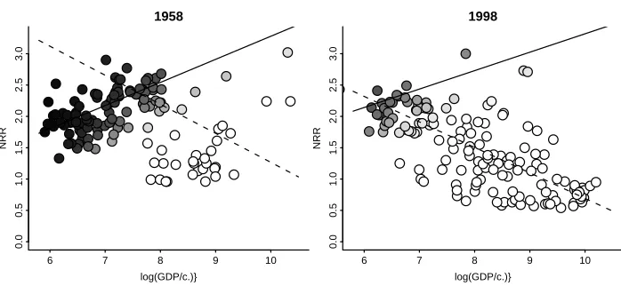
Figure 2: A graphical representation of the 1958 and 1998 estimations from Table 3; the Malthusian constraint is represented by the solid line, the demand for children by the dashed line; the gray scales denote the probabilities that an observation was determined by the de-mand for children (black:APi= 0, white:APi= 1)

6 7 8 9 10

0.0

0.5

1.0

1.5

2.0

2.5

3.0

1958

log(GDP/c.)}

NRR

6 7 8 9 10

0.0

0.5

1.0

1.5

2.0

2.5

3.0

1998

log(GDP/c.)}

NRR

By pooling the data, the shifts of the demand for children and the Malthusian con-straint may be analyzed over time. The resulting autocorrelation, which violates the assumption of independence of the residuals, should not be a matter of concern, as the number of points in time (10) is very low compared to the number of units (152). The fourth column in Table 3 reports the estimation of the switching regression model in a pooled sample. The results are very similar to the period-by-period regressions.

Specification (5) includes a time trend both for the demand and the constraint function. The time trend measures the number of years since 1953 (for example, in 1998, the time trend has a value of 45). In line with expectations, the constraint function moves upward over time, and the demand function moves downwards.8 _{On average, the Malthusian}

constraint relaxes by 0.013 NRR points per year, leading to an increase of 0.585 NRR points over the whole sample period. The demand for children decreases by 0.016 NRR points per year, leading to a decrease by 0.720 pairs of children over 45 years. Finally, instead of a time trend, specification (6) uses dummy variables for each point in time. Again, the coefficients for GDP per capita are very similar.

8_{Including a time-GDP interaction term—thereby allowing the slopes of the demand and the constraint}

(23)

5.2 Specific explanatory variables

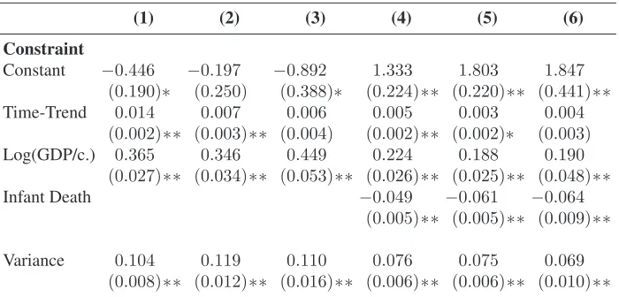
Thanks to its parametric nature, the switching regression framework allows the inclusion of additional variables. As mentioned above, including function-specific variables solves the identification problem. Table 4 shows some results with specific explanatory variables. The first specification includes three demand-specific variables: The ratio of Muslims, the ratio of Catholics and a dummy variable indicating whether a country is a major oil exporter or not. All three variables are significant and have the expected sign: other things being equal, the demand for children in a completely Muslim country is 0.638 NRR points higher than in a non-Muslim country. In a completely Catholic country, the same value is 0.407 compared to a non-Catholic country. Similarly, being heavily dependent on oil exports increases the demand for children by 0.756.

Table 4: The determinants of the NRR (2) — maximum likelihood estima-tion of the switching regression model; demand-specific explanatory variables (1) to (3); constraint-specific variables (4); specific vari-ables for both functions (5), (6). Standard errors from2nd

deriva-tives in parentheses; * significant at 5%, ** at 1%

(1) (2) (3) (4) (5) (6)

Constraint

Constant −0.446 −0.197 −0.892 1.333 1.803 1.847 (0.190)∗ (0.250) (0.388)∗ (0.224)∗∗ (0.220)∗∗ (0.441)∗∗ Time-Trend 0.014 0.007 0.006 0.005 0.003 0.004

(0.002)∗∗ (0.003)∗∗ (0.004) (0.002)∗∗ (0.002)∗ (0.003)

Log(GDP/c.) 0.365 0.346 0.449 0.224 0.188 0.190 (0.027)∗∗ (0.034)∗∗ (0.053)∗∗ (0.026)∗∗ (0.025)∗∗ (0.048)∗∗ Infant Death −0.049 −0.061 −0.064

(0.005)∗∗ (0.005)∗∗ (0.009)∗∗

(24)

Table 4: (Continued)

(1) (2) (3) (4) (5) (6)

Demand

Constant 5.700 5.659 4.895 6.309 5.859 4.689 (0.173)∗∗ (0.205)∗∗ (0.264)∗∗ (0.234)∗∗ (0.177)∗∗ (0.274)∗∗ Time-Trend −0.016 −0.021 −0.015 −0.014 −0.013 −0.015

(0.001)∗∗ (0.002)∗∗ (0.002)∗∗ (0.002)∗∗ (0.001)∗∗ (0.002)∗∗ Log(GDP/c.) −0.472 −0.419 −0.308 −0.498 −0.500 −0.277

(0.020)∗∗ (0.027)∗∗ (0.037)∗∗ (0.027)∗∗ (0.021)∗∗ (0.039)∗∗

School y. −0.077 −0.083

(0.012)∗∗ (0.013)∗∗

Urban −0.427 −0.097 −0.165

(0.104)∗∗ (0.112) (0.121)

Oil 0.756 0.798 0.501 0.793 0.562 (0.068)∗∗ (0.070)∗∗ (0.072)∗∗ (0.074)∗∗ (0.077)∗∗ Catholic 0.407 0.428 0.286 0.420 0.321

(0.046)∗∗ (0.047)∗∗ (0.052)∗∗ (0.048)∗∗ (0.055)∗∗ Muslim 0.638 0.651 0.429 0.770 0.484

(0.063)∗∗ (0.065)∗∗ (0.085)∗∗ (0.071)∗∗ (0.085)∗∗

Variance 0.208 0.181 0.152 0.381 0.202 0.152 (0.011)∗∗ (0.010)∗∗ (0.010)∗∗ (0.023)∗∗ (0.011)∗∗ (0.010)∗∗

Log-LL 630.06 481.29 292.06 721.01 470.59 228.75

n 1358 1090 762 1208 1208 664

(25)

the more parsimonious specifications, while the coefficient on urbanization still has the expected sign, but is not significant any more.

On the constraint function, the fourth specification includes the infant death rate. As expected, a higher rate tightens the Malthusian constraint. An increase in the infant death rate by one percent point tightens the constraint by about 0.05 NRR points.9 _Finally,

the two last specifications include the same demand-specific variables as in (1) to (3). Altogether, an inclusion of the infant death rate does not change the size of the demand coefficients significantly.

The last specification is the most extensive formulation. Its graphical representation is given in Figure 3. For ease of comparison, the observations are plotted in the same two dimensional GDP per capita and NRR space as in Figure 2. However, the calculated as-signment probabilities are based on the multivariate estimation of specification (6). While it is still true that poorer countries are more likely to have a constraint-determined fertility, there are interesting exceptions to the rule. Consider, for example, South Korea (KOR) and Liberia (LBR) in 1963 (all data for these countries can be found in Table 2). The GDP per capita was about the same in 1963 in both countries (Liberia: 1204 $, Korea: 1316 $), as was the Net Rate of Reproduction (Liberia: 2.05, Korea: 2.11). The sharp differences behind the superficial similarities are reflected in very different assignment probabilities. Liberia’s assignment probability in 1963 was 0.13, indicating that Liberia’s fertility was likely to be determined by the Malthusian constraint. On the other hand, Korea’s assignment probability was 0.97, indicating that Korea’s net fertility was almost surely determined by demand. These differences arise from differences in the explana-tory variables. Child mortality, for example, was much higher in Liberia than in in Korea, indicating a lower Malthusian constraint function in the latter country. On the other hand, the demand for children was likely to be lower in Korea than in Liberia, due to a higher level of education and a lower ratio of Muslim population.

9_{The infant death rate is used because its data has the same coverage as the NRR. However, one could argue}

(26)

Figure 3: A graphical representation of the assignment probabilities gener-ated from estimation (6) in Table 4; 1963 and 1993; the gray scales denote the probabilities that an observation was determined by the demand for children (black:APi= 0, white:APi = 1)

6 7 8 9 10

0.0

0.5

1.0

1.5

2.0

2.5

3.0

1963

log(GDP/c.)

NRR

6 7 8 9 10

0.0

0.5

1.0

1.5

2.0

2.5

3.0

1993

log(GDP/c.)

NRR

6. Conclusion

This paper estimates a simplified version of Easterlin’s supply-demand framework using a switching regression technique. In 1953, many poor countries had not yet completed the demographic transition. Accordingly, the determination of net fertility in these countries was very different than in post-transitional countries. Income, for example, generally had a positive impact on net fertility in poor countries, while it has a negative impact today. Easterlin’s supply-demand framework offers an explanation for this fact by attributing the positive relationship to Malthusian “supply” factors and the negative relationship to “demand” factors.

(27)

Several variables are found to affect the Malthusian constraint: Doubling non-logarithmic GDP per capita relaxes the constraint by between 0.3 and 0.5 surviving chil-dren. An increase in the infant death rate by one percentage point tightens the constraint by 0.1 surviving children. Over the whole sample period, the constraint relaxes by be-tween 0.3 and 1.6 surviving children. At the same time, doubling the non-logarithmic GDP per capita decreases the demand for children by between 0.4 and 0.7 surviving chil-dren. An additional year of education decreases the demand for children by about 0.16 surviving children. Also, the demand for children increases if a country has a high per-centage of Muslims (1.0 to 1.3) or Catholics (0.6 to 0.8), or if it is heavily depended on oil exports (1.1 to 1.5). The effect of urbanization on the demand for children is significantly negative in some specifications, but not in others.

Over time, a combination of higher GDP per capita, a decrease in the infant death rate and an increase in education explain part of the shift from the Malthusian constraint to the demand for children in many countries. In addition to that, there is an unexplained upward shift over time in the Malthusian constraint and a downward shift in the demand for children. The cumulation of these shifts is sufficient to explain the reversal of the relationship between income and the number of surviving children over the sample period. The shift from a Malthusian determination of net fertility to demand is one of the interesting and most relevant interpretations of the analysis. Malthusian factors, while important in 1953, relaxed over time and have lost their significance today; demand fac-tors, on the other hand, have become more important. This has an important implication for the analysis of fertility. While the inclusion of Malthusian factors, such as child mor-tality, is essential for a historical analysis of net fertility, it is less indispensable today. Obviously, Malthusian factors are irrelevant for most people’s fertility determination in developed countries, as their fertility is exclusively determined by demand. But also in many developing countries, net fertility overwhelmingly relies on demand factors.

(28)

7. Acknowledgements

(29)

References

Amemiya, T. (1974). A note on a Fair and Jaffee Model. Econometrica42(4): 759–762.

doi:10.2307/1913944.

Barro, R.J. and Lee, J.W. (2000). International data on educational attainment: Updates and implications. Cambridge, MA, USA: Center for International Development at Harvard University. (CID Working Paper 42).

Becker, G.S. (1960). An economic analysis of fertility. In: National Bureau of Eco-nomic Research (ed.).Demographic and Economic Change in Developed Countries. Princeton: Princeton University Press: 209–231. (NBER Conference Series vol 11). Becker, G.S. and Lewis, H.G. (1973). On the interaction between the quantity and quality

of qhildren.The Journal of Political Economy81(2): 279–288.doi:10.1086/260166. Becker, G.S. and Tomes, N. (1976). Child endowments and the quantity and quality of

children.The Journal of Political Economy84(4): 143–162.doi:10.1086/260536. Caldwell, J.C. (1976). Toward a restatement of demographic transition theory.Population

and Development Review2(3/4): 321–366. doi:10.2307/1971615.

Caldwell, J.C. (1980). Mass education as a determinant of the timing of fertility decline.

Population and Development Review6(2): 225–255.doi:10.2307/1972729.

Docquier, F. (2004). Income distribution, non-convexities and the fertility-income rela-tionship.Economica71(282): 261–273. doi:10.1111/j.0013-0427.2004.00369.x. Drèze, J.H. and Bean, C.R. (1988). Europe’s unemployment problem. Cambridge, USA:

MIT Press.

Easterlin, R.A. (1975). An economic framework for fertility analysis. Studies in Familiy Planning6(3): 54–63.doi:10.2307/1964934.

Easterlin, R.A. (1978). The economics and sociology of fertility: A synthesis. In: Tilly, C. (ed.).Historical Studies of Changing Fertility. Princeton University Press: 57–133. Fair, R.C. and Jaffee, D.M. (1972). Methods of estimation for markets in disequilibrium.

Econometrica40(3): 497–514.doi:10.2307/1913181.

Fernandez, R. and Fogli, A. (2006). Fertility: The role of culture and family experience. Journal of the European Economic Association 4(2-3): 552–561.

doi:10.1162/jeea.2006.4.2-3.552.

(30)

North-Holland: 172–293. (Vol 1A).

Galor, O. and Moav, O. (2003). Das Human Kapial – A theory of the demise of the class structure. Brown University. (Brown University Working Paper 2000-17).

Galor, O. and Weil, D.N. (1996). The gender gap, fertility, and growth. The American Economic Review86(3): 374–387.

Galor, O. and Weil, D.N. (1999). From malthusian stagnation to modern growth. The American Economic Review89(2): 150–154. doi:10.1257/aer.89.2.150.

Hazan, M. and Berdugo, B. (2002). Child labour, fertility, and economic growth. Eco-nomic Journal112(482): 810–828.doi:10.1111/1468-0297.00066.

Kalemli-Ozcan, S. (2003). A stochastic model of mortality, fertility, and hu-man capital investment. Journal of Development Economics 70(1): 103–118. http://www.sciencedirect.com/science/article/pii/S0304387802000895. doi:10.1016/S

0304-3878(02)00089-5.

Kiefer, N.M. (1980). A note on regime classification in disequilibrium models. The Review of Economic Studies47(3): 637–639.doi:10.2307/2297314.

La Porta, R., Lopez-de-Silanes, F., Shleifer, A., and Vishny, R. (1999). The qual-ity of government. Journal of Law, Economics, and Organization 15(1): 222–279.

doi:10.1093/jleo/15.1.222.

Lambert, J.P., Lubrano, M., and Sneessens, H.R. (1984). Emploi et chômage en France de 1955 à 1982: un modèle macroéconomique. annuel avec rationnement. Annales de l’INSEE55/56: 39–76.

Lee, R.D. (1987). Population dynamics of humans and other animals.Demography24(4): 443–465.doi:10.2307/2061385.

Maddala, G.S. (1983). Limited-Dependent and Qualitative Variables in Econometrics. Cambridge UK: Cambridge University Press.

Maddala, G.S. (1986). Disequilibrium, self-selection, and switching models. In: Griliches, Z. and Intriligator, M.D. (eds.).Handbook of Econometrics. Elsevier Sci-ence Publishers: 1634–1688. (Vol. 3, Ch. 28).

Maddala, G.S. and Nelson, F.D. (1974). Maximum Likelihood Methods for models of markets in disequilibrium.Econometrica42(6): 1013–1030.doi:10.2307/1914215. Maddison, A. (2003). Historical Statistics. Paris: OECD. (OECD Development Centre

Studies).

(31)

E.A. and Souden, D. (eds.).The Works of Thomas Robert Malthus. London: William Pickering. (Vol 1).

McQuillan, K. (2004). When does religion influence fertility? Population and Develop-ment Review30(1): 25–56. doi:10.1111/j.1728-4457.2004.00002.x.

Montgomery, M.R. (1987). A new look at the Easterlin “Synthesis” Framework. Demog-raphy24(4): 481–496. doi:10.2307/2061387.

Pritchett, L.H. (1994). Desired fertility and the impact of population policies.Population and Development Review20(1): 1–55.doi:10.2307/2137629.

Quandt, R.E. (1986). A note on estimating disequilibrium models with aggregation. Em-pirical Economics11(4): 223–242.doi:10.1007/BF01977003.

Quandt, R.E. (1988). The Econometrics of Disequilibrium. New York: Blackwell. Ross, M.L. (2001). Does oil hinder democracy? World Politics 53(03): 325–361.

doi:10.1353/wp.2001.0011.

Schapiro, M.O. (1982). Land availability and fertility in the United States, 1760-1870.

The Journal of Economic History42(3): 577–600. doi:10.1017/S0022050700027960. Shapiro, D. and Tambashe, B.O. (2001). Fertility in the Democratic Republic of the

Congo. Population Research Institute, Pennsylvania State University. Simonoff, J.S. (1996). Smoothing methods in statistics. New York: Springer.

Stys, W. (1957). The influence of economic conditions on the fertility of peasant women.

Population Studies11(2): 136–148.doi:10.2307/2172109.

United Nations Statistics Division (2001). Demographic Yearbook, Historical Supple-ment, 1948-1997. [CD-ROM].

Weir, D.R. (1995). Family income, mortality, and fertility on the eve of the demographic transition: A case study of Rosny-Sous-Bois. Journal of Economic History55(1): 1–

26.doi:10.1017/S0022050700040559.

(32)

A Appendix

A1 An expression for the assignment probability

With the estimations of the parameter at hand, the probability that an observation belongs either to the demand or to the constraint can be calculated. Kiefer (1980) proposed the calculation of the following expression:

APi= Pr(nCi< nDi|nAi) (13)

Using the Bayes formula,

Pr(A|B) = Pr(B|A)·Pr(A) Pr(B)

Eq. (13) can be written as:

Pr(nCi< nDi|nAi) = Pr(nAi|nCi< nDi)·Pr(nCi< nDi)

P r(nAi)

= h(nAi|nCi< nDi)·Πi

h(nAi)

Using Eq. (11), this can be written as:

Pr(nCi< nDi|nAi) = Z _∞

nAi

g(nAi, nDi)dnDi/h(nAi)

= fC(nAi)(1−FD(nAi))

fD(nAi)(1−FC(nAi)) +fC(nAi)(1−FD(nAi))(14)

(33)

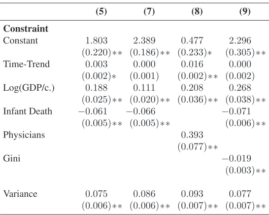
A2 Additional estimations

Table 5: The determinants of the NRR (3) — maximum likelihood esti-mation of the switching regression model; benchmark estiesti-mation from table 4 (5); infant death rate on the demand side (7); num-ber of physicians as a proxy for Malthusian conditions (8); Gini-coefficients in both functions (9). Standard errors from2nd

deriva-tives in parentheses; * significant at 5%, ** at 1%

(5) (7) (8) (9)

Constraint

Constant 1.803 2.389 0.477 2.296 (0.220)∗∗ (0.186)∗∗ (0.233)∗ (0.305)∗∗ Time-Trend 0.003 0.000 0.016 0.000