DEMOGRAPHIC RESEARCH
VOLUME 31, ARTICLE 30, PAGES 913940
PUBLISHED 17 OCTOBER 2014
http://www.demographic-research.org/Volumes/Vol31/30/ DOI: 10.4054/DemRes.2014.31.30
Research Article
An empirical analysis of the importance of
controlling for unobserved heterogeneity when
estimating the income-mortality gradient
Adriaan S. Kalwij
©2014 Adriaan S. Kalwij.
This open-access work is published under the terms of the Creative Commons Attribution NonCommercial License 2.0 Germany, which permits use, reproduction & distribution in any medium for non-commercial purposes, provided the original author(s) and source are given credit.
1 Introduction 914
2 Individual mortality risk model 917
2.1 Model identification and assumptions 918
2.2 Assumption of no unobserved heterogeneity 919 2.3 Assumption of a gamma distribution for unobserved heterogeneity 920
3 Empirical analysis 920
3.1 The data 920
3.2 Empirical model 922
3.3 Empirical results 922
4 Conclusions 925
References 927
An empirical analysis of the importance of controlling for
unobserved heterogeneity when estimating the income-mortality
gradient
Adriaan S. Kalwij1
Abstract
BACKGROUND
Statistical theory predicts that failing to control for unobserved heterogeneity in a Gompertz mortality risk model attenuates the estimated income-mortality gradient toward zero.
OBJECTIVE
I assess the empirical importance of controlling for unobserved heterogeneity in a Gompertz mortality risk model when estimating the income-mortality gradient. The analysis is carried out using individual-level administrative data from the Netherlands over the period 1996–2012.
METHODS
I estimate a Gompertz mortality risk model in which unobserved heterogeneity has a gamma distribution and left-truncation of life durations is explicitly taken into account.
RESULTS
I find that, despite a strong and significant presence of unobserved heterogeneity in both the male and female samples, failure to control for unobserved heterogeneity yields only a small and insignificant attenuation bias in the negative income-mortality gradient.
CONCLUSIONS
The main finding, a small and insignificant attenuation bias in the negative income-mortality gradient when failing to control for unobserved heterogeneity, is positive news for the many empirical studies, whose estimations of the income-mortality gradient ignore unobserved heterogeneity.
1
1. Introduction
The main contribution of this paper to the literature is to statistically test the empirical importance for the income-mortality gradient of controlling for unobserved heterogeneity in a Gompertz mortality risk model. Statistical theory predicts that failing to control for unobserved heterogeneity attenuates the estimated income-mortality gradient toward zero. Using individual-level administrative data from the Netherlands, I estimate a Gompertz mortality risk model in which unobserved heterogeneity has a gamma distribution, taking into account left-truncation of life durations due to individuals only entering the sample after age 65. The main finding is that for both men and women, unobserved heterogeneity is strongly and significantly present, but that failing to control for it does not significantly attenuate the income-mortality gradient toward zero.
Empirical studies covering many populations and time periods have found a strong and significant inverse relationship between income and mortality risk.2 This negative income-mortality gradient, a dimension of the health gradient by socioeconomic status, has important implications for economic and public health policies (Brown 2000; Huisman et al. 2005; Menchik 1993; Nelissen 1999; Whitehouse and Zaidi 2008). Most particularly, it suggests a need for public health interventions to reduce health risk factors in low-income groups. Suggestions for economic policy vary from using welfare programs to alleviate poverty, and thereby possibly improve health in low-income groups, to addressing the issue that financial products such as uniformly priced private pension plans have a lower (higher) internal rate of return for low (high)-income groups as they have lower (higher) life expectancy.
The standard empirical framework for estimating the income-mortality gradient is a hazard rate model, in which individual mortality risk is explained by age, income, and possibly other covariates. In any empirical analysis of mortality risk, however, a sample of individuals inherently becomes more selected with age in terms of both observed and unobserved individual characteristics (Vaupel and Yashin 2006). Time-invariant unobserved individual characteristics (hereafter, unobserved heterogeneity) are, for instance, related to individual differences in longevity endowment, such as genes (Robine 2007), macroeconomic conditions around birth (Van den Berg, Lindeboom, and Portrait 2006), parents’ socioeconomic status (Flores and Kalwij 2014) or even prenatal circumstances (Barker 1995).
Statistical theory predicts that failing to control for unobserved heterogeneity in a mortality model with a proportional hazard specification attenuates the estimated
2 See Blakely et al. (2004) for New Zealand, Duleep (1986) for the U.S., Gaudecker and Scholz (2007) for
(positive) age and covariate effects toward zero (Bretagnolle and Huber-Carol 1988; Aalen 1994; Chamberlain 1985; Lancaster 1990; Schumacher, Olschewski, and Schmoor 1987). The consequences of ignoring such unobserved heterogeneity in the age-mortality gradient has received much attention in the literature following a seminal paper by Vaupel, Manton, and Stallard (1979) that refers to unobserved heterogeneity as “frailty”. Although Vaupel, Manton, and Stallard’s (1979) work sparked many studies – including Congdon (1994), Hougaard (1984), Manton, Stallard, and Vaupel (1981; 1986) and Vaupel and Yashin (1985) – these are mostly concerned with life tables for heterogeneous populations.3 This research does show that, as predicted by statistical theory, the positive age-mortality gradient is steeper once unobserved heterogeneity is taken into account. Studies in other disciplines, including economics and medicine, have also acknowledged the potential importance of controlling for unobserved heterogeneity when investigating, for example, the duration dependence of a hazard rate in such varied topics as birth timing, unemployment episodes, and clinical trials (see Heckman and Singer 1982; Lancaster 1979; Newman and McCulloch 1984; Shepard and Zeckhauser 1980; Turnbull, Jiang, and Clark 1997).
Yet despite the importance of the income-mortality gradient for policymakers, and considering the clear statistical predictions on the consequences of ignoring unobserved heterogeneity in a mortality risk model, little empirical evidence is available on the size of the attenuation bias in the income-mortality gradient when failing to control for unobserved heterogeneity.4 In particular, failing to control for unobserved heterogeneity results in an attenuation of the impact of income on mortality toward zero and policymakers may therefore underestimate its association with mortality. To my knowledge, only a handful of empirical papers provide some insight into this issue. Among these, Congdon (1994), using data from London boroughs, shows that allowing for unobserved heterogeneity does not markedly affect the association between mortality and a measure of deprivation. Likewise, Frijters, Shields, and Haisken-DeNew (2011), drawing on German data, identify only a less-than-half standard error difference in estimates of the household income-mortality link between models that do and do not control for unobserved heterogeneity. More recently, Kalwij, Alessie, and Knoef (2013) show a relatively small impact of not controlling for unobserved heterogeneity on the estimated associations between individual and spousal income and mortality risk in the Netherlands. These findings echo Omariba, Beaujot, and Rajulton’s (2007) conclusion that failure to control for unobserved heterogeneity barely affects the impact of household income (among other factors) on infant and child mortality in
3 These and the many related studies often investigate the flattening of mortality risk at older ages or mortality
among the oldest old. Allied to this research are correlated and shared frailty models (not discussed here) that often use data on twins to examine the role of genes in longevity (Yashin, Iachine, and Harris 1999).
4
Kenya. In sum, although unobserved heterogeneity is significantly present in all four studies, not one suggests that failing to model unobserved heterogeneity yields a large attenuation bias in the estimated income-mortality gradient.
These studies, however, share a common methodological shortcoming: they do not take into account the left-truncation of life durations that is inherent to using a stock sample with information on remaining life durations for those who have survived up to the survey year (i.e. a non-random sample). In fact, both Congdon (1994) and Omariba, Beaujot, and Rajulton (2007) ignore it, while Frijters, Shields, and Haisken-DeNew (2011) and Kalwij, Alessie, and Knoef (2013) take it to some extent into account in a heuristic way by adding to their models, respectively, health status and interactions between the covariates and age in the year of first observation. Yet not accounting for left truncation yields inconsistent estimates in mortality risk models in which unobserved heterogeneity is present (Lancaster 1990; Ridder 1984) and may influence comparisons of estimated income-mortality gradients between models that have and do not have controlled for unobserved heterogeneity.
The contribution of this paper to the empirical literature is twofold. First, I take into account the left truncation of life durations in a mortality risk model with unobserved heterogeneity that is used to estimate the income-mortality gradient. Second, I not only quantify the attenuation bias in the income-mortality gradient that is generated by ignoring unobserved heterogeneity, but also test its significance, a step not taken in previous studies. For reasons of identification (explicated below), I restrict most of the analysis to one model widely used in the related empirical literature: a Gompertz model in which unobserved heterogeneity has a gamma distribution. The empirical analysis is carried out using individual-level administrative data from the Netherlands over the period 1996–2012.
2. Individual mortality risk model
In line with most of the studies cited above, I assume that individual mortality risk at age T= t conditional on observed covariates x and unobserved heterogeneity θ is given by
( | ) ( ) ( ) with (1) where α is a vector determining the age pattern of individual mortality risk and β is a parameter vector determining the relation between the covariates and individual mortality risk. Unobserved heterogeneity θ is an unobserved time-constant individual characteristic, ( | ) is a hazard rate, and the covariates are modeled in the multiplicative manner often termed a proportional hazard specification (Cox 1972).
As in most previous studies, the estimation of the parameter vectors α and β is based on a stock sample containing information on the calendar time at which the individual entered the current state (birth date), the age when entering the sample, and either the life duration (age of death) or the duration until the end of the observation period (a right-censored observation). Because the probability of being in the sample (i.e., remaining alive until the sample start date) is inversely related to mortality risk, the stock sample is a non-random sample. Estimation is thus based on a conditional likelihood that takes into account the left-truncation of life durations in the sample. The truncated density function of a completed duration t conditional on entering the sample at age t0 (and on x) is given by equation (2) (see Online Supplementary Appendix A):
̃ ( | ) ∫ ( | ) ( )
∫ ( | ) ( ) (2)
where ( | ) is the probability density function of a life duration, ( | ) is the survivor function (i.e., the probability of being alive at a certain age), and ( ) is the probability density function of unobserved heterogeneity with parameter vector γ. The left-truncated distribution function of an incomplete life duration t (i.e., a right-censored observation) conditional on entering the sample at age t0 is given by
̃ ( | ) ∫ ( | ) ( )
∫ ( | ) ( ) (3)
likelihood estimator (CMLE) based on a stock sample of N individuals is given as follows (see Online Supplementary Appendix A):
∑ ( ̃ ( | ))
( ) ( ̃( | ))
(4)
Here, the variable mi is equal to one if individual i’s duration is complete (dead) and to
zero if incomplete (alive; right censored).
2.1 Model identification and assumptions
Elbers and Ridder (1982) prove the nonparametric identification of both a hazard rate’s duration dependence and the unobserved heterogeneity distribution when assuming the multiplicative specification formalized in equation (1).5 Such identification is, however, impossible using a left-truncated sample and an assumption is needed concerning the distribution of unobserved heterogeneity.6
Following Vaupel, Manton, and Stallard (1979), the demographic literature on mortality risk often assumes a gamma distribution and, moreover, Abbring and Van den Berg (2007) and Missov and Finkelstein (2011) provide a theoretical justification for using this distribution. I therefore assume that unobserved heterogeneity has a gamma distribution. Nevertheless, in the empirical analysis I also use, as a sensitivity analysis, a log-normal and an inverse Gaussian distribution for unobserved heterogeneity.
In modeling the age-mortality relationship, I assume a Gompertz specification and allow the inclusion of only time-constant observed covariates, thereby enabling explicit modeling of the left-truncation, i.e. survival up to the age of sample entry (see Online Supplementary Appendix A).7 This modeling is based on predicted mortality risks at
5 Elbers and Ridder (1982) prove that, in this case, the densities of duration (conditional on unobserved
heterogeneity) and unobserved heterogeneity are separately and non-parametrically identified from observed individuals’ (incomplete) durations when the risk model contains at least one continuous covariate and an assumption concerning either the first moment (needs to be finite) or the tail behavior of the mixing distribution. A semi-parametric estimator is provided in Horowitz (1999).
6 Using the Kuhn-Tucker approach of Baker and Melino (2000), it can be shown that applying a
Non-Parametric MLE estimator (Heckman and Singer 1984) to a left-truncated sample of durations causes a non-identification of the probability distribution function of unobserved heterogeneity.
7
younger ages, which requires the functional form assumption of a Gompertz specification for the age-dependency of mortality risk. I return to this in section 3.3.
2.2 Assumption of no unobserved heterogeneity
An assumption of no unobserved heterogeneity simplifies model estimation and eliminates the need to make the identifying assumptions discussed in section 2.1. In this case, the CMLE is given by (see Online Supplementary Appendix C)
∑ ( ( | ))
∫ ( | )
(5)
where ( | ) ( ) ( ). Admittedly, this assumption of no unobserved heterogeneity is inconsistent with a mortality risk model’s inherent feature: that with age, the sample of survivors is an endogenously selected sample on both observed and unobserved characteristics. Nevertheless, in empirical studies on whether a characteristic is positively or negatively correlated with mortality risk – in which a statistical test would produce a bias toward not rejecting the null hypothesis of no effect (Lancaster 1990, Chap. 4) – this assumption might be preferable to those outlined in section 2.1. A study that ignores unobserved heterogeneity in a proportional hazard rate model and rejects the null-hypothesis of no association between a characteristic and mortality risk, would also reject the null-hypothesis once unobserved heterogeneity is controlled for.8
8
2.3 Assumption of a gamma distribution for unobserved heterogeneity
As explained above, I assume for the most part of the analysis that the unobserved heterogeneity distribution ( ) is a gamma distribution. Online Supplementary Appendix C derives the necessary likelihood contributions, which yield the following CMLE:
∑ (
( ) ( ) ( ) ( ))
(( ( ) ( ) ( ) ( ))
)
(6)
where ( ) ∫ ( ) and is the variance of unobserved heterogeneity.
3. Empirical analysis
3.1 The data
The data are drawn from the 1996–2010 Income Panel Study of the Netherlands (IPO, Inkomens Panel Onderzoek, CBS 2012a) and the 1997–2012 Causes of Death Registry (DO, Doodsoorzaken, CBS 2012b), both gathered by Statistics Netherlands. The IPO, a representative sample of the Dutch population, consists of an administrative panel dataset of about 95,000 selected individuals (per year on average) who are followed longitudinally. Sampling is based on each individual’s national security number, and the selected individuals are followed for as long as they are residing in the Netherlands on December 31 of the sample year. Individuals only exit the panel on death or emigration from the Netherlands.9
The IPO contains data on gender, year and birth month, and household income, all obtained from official institutions such as the population registry, tax office, and agencies that pay out (insurance) benefits. The DO, on the other hand, provides the date of death for all residents deceased during the 1997–2012 period, taken from records provided by medical examiners, who are legally obliged to submit them to Statistics Netherlands. The DO dataset also assigns a personal identifier, which allows determination of whether an individual in the IPO has died and, if so, when.
I select individuals from the IPO sample who are aged 65 or older on December 31 in one of the years in the 1996–2010 period (about 14 percent of the sample) and follow them from the age of sample entry until either death or the end of the sample period, whichever comes first.10 I choose 65 as a minimum age because in the Netherlands it is the statutory retirement age at which labor contracts are terminated and unemployment, disability, and assistance benefits cease. After age 65, all individuals receive a public pension benefit (independent of past earnings) and an occupational pension that depends on earnings history (Nelissen 1999). Because this retirement income consists primarily of pension income – and is thus closely related to earnings history – it serves as a good proxy for the socioeconomic status dimension, lifetime income. Because of missing income information, I remove 1.1 percent of the observations, leaving a final sample of 5,193 men and 7,681 women.
The dependent variable in the analysis is life duration measured in months. As shown in table 1, during the observation period, 3,809 men and 5,114 women die, at an average age of 82 years for men and 86 years for women. On average, men enter the sample at age 74 and women at age 76. The only covariate used in this analysis is standardized household income (referred to as “income”), measured in the year of sample entry, and is defined as disposable household income – that is, net of taxes and social insurance contributions – measured in 2010 euros using the consumer price index and divided by the equivalence scale provided by Statistics Netherlands (Siermann, van Teeffelen, and Urlings 2004).
Table 1: Sample statistics
Men Women
Number of individuals 5193 7681
Average income (in euros) 19967 18174
Income, 25th percentile (in euros) 13159 12372
Income, 50th percentile (in euros) 16614 15129
Income, 75th percentile (in euros) 23543 21595
Average age at entry (into the sample) 74 76
Number of deaths 3809 5114
Average age at death (for those who have died) 82 86
3.2 Empirical model
In his seminal article Gompertz (1825) characterizes the way that mortality risk changes with age (Gompertz law of mortality) and I formalize this concept in my proportional hazard specification (equation (1)) as an exponential increase in mortality risk with age. I further assume that the logarithm of income proportionally affects mortality risk (i.e. a constant income elasticity of mortality risk) and include calendar time (measured in months) to control for mortality trends. I thus specify individual mortality risk as
( | ) ( ( )) (7) I estimate this mortality model using five different empirical specifications. The first, a Cox model (Cox 1972) using partial maximum likelihood (model 1), is semi-parametric in that it does not make a functional form assumption about the age-mortality gradient. However, it identifies the parameters β1 and β2 of equation (7) under
the assumption of no unobserved heterogeneity (i.e., that θ is equal to 1 for all individuals). This model is widely used, in particular in the epidemiological literature, and given it’s flexible age-mortality relation, a comparison of the estimated income-mortality gradient with the one from a Gompertz model will show if the restrictive specification of the age-mortality relation in a Gompertz model affects the income-mortality gradient. The other four models are Gompertz models. Model 2 does not control for unobserved heterogeneity (see section 2.2) and model 3 includes gamma distributed unobserved heterogeneity (see section 2.3). I investigate the sensitivity of the estimated income-mortality gradient with respect to the choice of the unobserved heterogeneity distribution by using as well a log-normal and an inverse Gaussian distribution (models 4 and 5).11
3.3 Empirical results
As Table 2 shows, for both men and women, the estimates of the time and income effects are virtually identical in models 1 and 2, suggesting that in research focused on the income-mortality gradient, the results are likely not to be influenced by using a Gompertz age-mortality gradient specification in a proportional hazard rate model. As predicted by statistical theory, controlling for gamma-distributed, unobserved heterogeneity results in stronger estimated age-mortality and income-mortality gradients for both men and women (model 3 vs. model 2). When using an inverse Gaussian distribution for unobserved heterogeneity (model 5) the results are rather
similar to those achieved when using a gamma distribution. When using the log-normal distribution (model 4) no significant unobserved heterogeneity is identified for men. Models 4 and 5 perform worse than model 3 in terms of fitting the data based on an Akaike Information Criterion (AIC). This result fits with the theoretical studies discussed in section 2.1 and in the remainder of this paper I consider only the gamma distribution for unobserved heterogeneity. Finally, the table shows that for all models the income-mortality gradient is about the same for men and women, and the decrease in mortality with calendar time is stronger for men than for women.
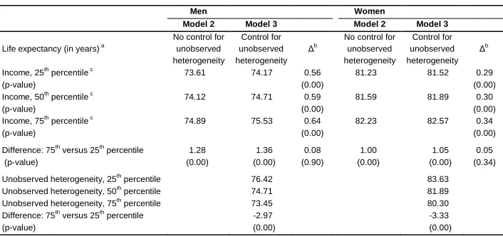
In model 3, the estimated variance of unobserved heterogeneity is equal to 0.068 for men and 0.1 for women, which is, by and large, in the range found in previous studies on adult mortality, even those that use different methodologies and fail to (properly) account for left-truncation. Congdon (1994), for instance, reports variances ranging from insignificantly different from zero, up to 0.13 (on average 0.043), Bissonnette (2012) finds a variance of 0.082 for U.S. men, and Kalwij, Alessie, and Knoef (2013) report a variance of 0.13 for men and 0.05 for women in the Netherlands. I next examine whether the underestimation in the income-mortality gradient when unobserved heterogeneity is not controlled for – about 15 percent for both men and women (model 2 vs. model 3) – leads to statistically significant differences in this gradient. To this end, table 3 reports life expectancies at the 25th, 50th, and 75th percentiles of the income and unobserved heterogeneity distributions and, more important, the differences in life expectancies for individuals with different levels of income and unobserved heterogeneity. As discussed in section 2.1, for the computation of life expectancy at birth I rely on the Gompertz specification, as it requires predictions of mortality risks at ages below 65 (out of sample). As regards the income-mortality gradient, in model 3, men with an income at the 25th percentile of the distribution have a 1.36 years shorter life expectancy than men with an income at the 75th percentile, a difference that is slightly lower (1.05 years) for women. Nevertheless, even though comparing these differences with those in model 2 shows that not controlling for unobserved heterogeneity yields smaller figures (1.28 years for men and 1 year for women), the attenuation biases are not only rather small (0.08 years for men and 0.05 years for women in model 2) but are insignificantly different from zero.
Table 2: Estimation results
Note: UH= Unobserved Heterogeneity.
a) UH is Gamma distributed in model 3, log-normally distributed in model 4 and inverse-Gaussian distributed in model 5. The
expectation of UH is normalized to one.
b) A Likelihood-Ratio test. Model 2 is the null-hypothesis (H0: no UH), against models 3, 4 or 5.
c) Akaike Information Criterion (AIC=2k-2xlog-likelihood; k=number of parameters; Akaike 1974). For the AIC calculations I
use unrounded log-likelihood values.
Table 3: Life expectancies in 1996 based on the estimation results of models 2 and 3 of Table 2
Men Women
Model 2 Model 3 Model 2 Model 3
Life expectancy (in years) a
No control for unobserved heterogeneity
Control for unobserved heterogeneity
Δb
No control for unobserved heterogeneity
Control for unobserved heterogeneity
Δb
Income, 25th
percentile c
73.61 74.17 0.56 81.23 81.52 0.29
(p-value) (0.00) (0.00)
Income, 50th
percentile c
74.12 74.71 0.59 81.59 81.89 0.30
(p-value) (0.00) (0.00)
Income, 75th
percentile c
74.89 75.53 0.64 82.23 82.57 0.34
(p-value) (0.00) (0.00)
Difference: 75th versus 25th percentile 1.28 1.36 0.08 1.00 1.05 0.05
(p-value) (0.00) (0.00) (0.90) (0.00) (0.00) (0.34)
Unobserved heterogeneity, 25th
percentile 76.42 83.63
Unobserved heterogeneity, 50th
percentile 74.71 81.89
Unobserved heterogeneity, 75th
percentile 73.45 80.30
Difference: 75th versus 25th percentile -2.97 -3.33
(p-value) (0.00) (0.00)
a
Only for a rough comparison: the Human Mortality Database (2008) reports a 1996 life expectancy of 74.65 for men and 80.33 for women.
b Δ is the difference in outcome between the model with and the model without controlling for unobserved heterogeneity.
c
Table 1 reports the 25th, 50th, and 75th percentiles of the income distribution.
4. Conclusions
My primary analytical concern in this paper is the extent to which the estimated income-mortality gradient is attenuated toward zero, when a Gompertz mortality risk model fails to control for unobserved heterogeneity. I do in fact identify a strong and significant presence of unobserved heterogeneity for both men and women, and find that, as statistical theory predicts, failing to control for unobserved heterogeneity attenuates the income-mortality gradient toward zero. Nevertheless, this attenuation bias is small and insignificantly different from zero, which is positive news for the large body of research on the income-mortality gradient that ignores unobserved heterogeneity.
risks at younger ages. In addition, the main finding is conditional on the Gompertz model with gamma-distributed unobserved heterogeneity. I have shown the robustness of my results when using different specifications, and more model selection tests and sensitivity analyses along these lines could be carried out. A potential limitation concerning the empirical specification is the constant income-mortality risk elasticity, and one may investigate a more flexible relationship between income and mortality risk (see, e.g., Belloni et al. 2013). Finally, future research might, for example, examine the importance of unobserved heterogeneity in the relationship between mortality and socioeconomic and behavioral risk variables, such as education and smoking behavior.12
References
Aalen O.O. (1994). Effects of frailty in survival analysis. Statistical Methods in Medical Research 3(3): 227–243. doi:10.1177/096228029400300303.
Abbring, J.H. and van den Berg, G.J. (2007). The unobserved heterogeneity distribution in duration analysis. Biometrika 94(1): 87–99. doi:10.1093/biomet/asm013. Akaike, H. (1974). A new look at the statistical model identification. IEE Transactions
on Automatic Control 19(6): 716–723. doi:10.1109/TAC.1974.1100705.
Baker, M. and Melino, A. (2000). Duration dependence and nonparametric heterogeneity: A Monte Carlo study. Journal of Econometrics 96(2): 357–393.
doi:10.1016/S0304-4076(99)00064-0.
Barker, D.J.P. (1995). Fetal origins of coronary heart disease. British Medical Journal 311(6998): 171–174. doi:10.1136/bmj.311.6998.171.
Belloni, M., Alessie, R.J.M., Kalwij, A.S., and Marinacci, C. (2013). Lifetime income and old-age mortality risk in Italy over two decades. Demographic Research 29(45): 1261–1298. doi:10.4054/DemRes.2013.29.45.
Bissonnette, L. (2012). Essays on subjective expectations and stated preferences. [Ph.D. Thesis]. Tilburg University.
Blakely, T., Kawachi, I., Atkinson, J., and Fawcett, J. (2004). Income and mortality: The shape of the association and confounding New Zealand Census – Mortality Study, 1981–1999. International Journal of Epidemiology 33(4): 874–883.
doi:10.1093/ije/dyh156.
Bretagnolle, J. and Huber-Carol, C. (1988). Effects of omitting covariates in Cox’s model for survival data. Scandinavian Journal of Statistics 15(2): 125–138. Brown, J.R. (2000). Differential mortality and the value of individual account
retirement annuities. NBER Working Paper No. 7560. National Bureau of Economic Research, Cambridge, MA.
CBS Centraal Bureau voor de Statistiek (2012a). Documentatierapport Inkomenspanel onderzoek (IPO). Centrum voor Beleidsstatistiek, Voorburg.
Chamberlain, G. (1985). Heterogeneity, Omitted Variable Bias, and Duration Dependence. In: Heckman, J.J. and Singer, B.S. (eds.). Longitudinal Analysis of Labor Market Data. Cambridge: Cambridge University Press: 3–38. doi:10.10 17/CCOL0521304539.001
Congdon, P. (1994). Analysing mortality in London: Life-tables with frailty. Journal of the Royal Statistical Society. Series D (The Statistician) 43(2): 277–308. doi:10. 2307/2348345.
Cox, D.R. (1972). Regression models and life-tables. Journal of the Royal Statistical Society, Series B (Statistical Methodology) 34(2): 187–220.
D’Addio, A.C. and Rosholm, M. (2002). Left-censoring in duration data: Theory and applications. Working Paper No. 2002–5, University of Aarhus, Denmark. Duleep, H.O. (1986). Measuring income’s effect on adult mortality using longitudinal
administrative record data. Journal of Human Resources 21(2): 238–251.
doi:10.2307/145800.
Elbers, C. and Ridder, G. (1982). True and spurious duration dependence: The identifiability of the proportional hazard model. Review of Economic Studies 49(3): 403–409.
Flores, M. and Kalwij, A.S. (2014). The associations between early life circumstances and later life health and employment in Europe. Empirical Economics. forthcoming. doi:10.1007/s00181-013-0785-3.
Frijters, P., Shields, M.A., and Haisken-DeNew, J.P. (2011). The increasingly mixed proportional hazard model: An application to socioeconomic status, health shocks, and mortality. Journal of Business and Economic Statistics 29(2): 271–281. doi:10.1198/jbes.2010.08082.
Gaudecker, von H.M. and Scholz, R.D. (2007). Differential mortality by lifetime earnings in Germany. Demographic Research 17(4): 83–108. doi:10.4054/Dem Res.2007.17.4.
Gompertz, B. (1825). On the Nature of the Function Expressive of the Law of Human Mortality, and on a New Mode of Determining the Value of Life Contingencies. Philosophical Transactions of the Royal Society of London 115: 513–585.
doi:10.1098/rstl.1825.0026.
Heckman, J.J. and Singer, B. (1982). Population heterogeneity in demographic models. In: Land, K.C. and Rogers, A. (eds.). Multidimensional mathematical demography. New York: Academic Press: 567–599. doi:10.1016/B978-0-12-435640-5.50018-3.
Heckman, J.J. and Singer, B. (1984). A method for minimizing the impact of distributional assumptions in econometric models for duration data. Econometrica 52(2): 271–320. doi:10.2307/1911491.
Horowitz, J.L. (1999). Semi-parametric estimation of a proportional hazard rare model with unobserved heterogeneity. Econometrica 67(5): 1001–1028. doi:10.1111/ 1468-0262.00068.
Hougaard, P. (1984). Life table methods for heterogeneous populations: Distributions describing the heterogeneity. Biometrika 71(1): 75–83. doi:10.1093/biomet/71. 1.75.
Huisman, M., Kunst, A.E., Bopp, M., Borgan, J.-K., Borrell, C., Costa, G., Deboosere, P., Gadeyne, S., Glickman, M., Marinacci, C., Minder, C., Regidor, E., Valkonen, T., and Mackenbach, J.P. (2005). Educational inequalities in cause-specific mortality in middle-aged and older men and women in eight Western European populations. Lancet 365(9458): 493–500. doi:10.1016/S0140-6736 (05)17867-2.
Human Mortality Database (2008). Available at http://www.mortality.org.
Kalwij, A.S., Alessie, R.J.M., and Knoef, M.G. (2013). Individual income and remaining life expectancy at the statutory retirement age of 65 in the Netherlands. Demography 50(1): 181–206. doi:10.1007/s13524-012-0139-3. Lancaster, T. (1979). Econometric methods for the duration of unemployment.
Econometrica 47(4): 939–956. doi:10.2307/1914140.
Lancaster, T. (1990). The econometric analysis of transition data. Cambridge: Cambridge University Press.
Leombruni, R., Richiardi, M., Demaria, M., and Costa, G. (2010). Aspettative di vita, lavori usuranti ed equità del sistema previdenziale. Prime evidenze dal Work Histories Italian Panel. Epidemiologia e Prevenzione 34(4): 150–158.
Manton, K.G., Stallard, E., and Vaupel, J.W. (1981). Methods for comparing the mortality experiences of heterogeneous populations. Demography 18(3): 389–410. doi:10.2307/2061005.
Manton, K.G., Stallard, E., and Vaupel, J.W. (1986). Alternative models for the heterogeneity of mortality risks among the aged. Journal of the American Statistical Society 81(395): 635–644. doi:10.1080/01621459.1986.10478316. Martikainen, P., Mäkelä, P., Koskinen, S., and Valkonen, T. (2001). Income differences
in mortality: A register-based follow-up study of three million men and women. International Journal of Epidemiology 30(6): 1397–1405. doi:10.1093/ije/30.6. 1397.
Menchik, P.L. (1993). Economic status as a determinant of mortality among Black and White older men: Does poverty kill? Population Studies 47(3): 427–436.
doi:10.1080/0032472031000147226.
Missov, T.I. and Finkelstein, M. (2011). Admissible mixing distributions for a general class of mixture survival models with known asymptotics. Theoretical Population Biology 80(1): 64–70. doi:10.1016/j.tpb.2011.05.001.
Nelissen, J.H.M. (1999). Mortality differences related to socioeconomic status and the progressivity of old-age pensions and health insurance: The Netherlands. European Journal of Population 15(1): 77–97. doi:10.1023/A:1006188911462. Newman, J.L. and McCulloch, C.E. (1984). A hazard rate approach to the timing of
births. Econometrica 52(4): 939–961. doi:10.2307/1911192.
Omariba, D.W.R, Beaujot, R., and Rajulton, F. (2007). Determinants of infant and child mortality in Kenya: An analysis controlling for frailty. Population Research Policy Review 26(3): 299–321. doi:10.1007/s11113-007-9031-z.
Osler, M., Prescott, E., Grønbæk, M., Christensen, U., Due, P., and Engholm, G. (2002). Income inequality, individual income, and mortality in Danish adults: Analysis of pooled data from two cohort studies. British Medical Journal 324(7328): 13–16. doi:10.1136/bmj.324.7328.13.
Robine, J.-M. (2007). Research issues on human longevity. In: Robine, J.-M., Crimmins, E.M., Horiuchi, S., and Yi, Z. (eds.). Human longevity, individual life duration, and the growth of the oldest-old population. Dordrecht: Springer: 7–42. doi:10.1007/978-1-4020-4848-7_1.
Schumacher, M., Olschewski, M., and Schmoor, C. (1987). The impact of heterogeneity on the comparison of survival times. Statistics in Medicine 6(7): 773–784. doi:10.1002/sim.4780060708
Shepard, D.S. and Zeckhauser, R.K. (1980). Long-term effects of interventions to improve survival in mixed populations. Journal of Chronic Diseases 33(7): 413–433. doi:10.1016/0021-9681(80)90039-9.
Siermann, C., van Teeffelen, P., and Urlings, L. (2004). Equivalentiefactoren 1995– 2000: Methode en belangrijkste uitkomsten. Sociaal-economische Trends 3: 63–66.
Snyder, S.E. and Evans, W.N. (2006). The effect of income on mortality: Evidence from the social security notch. Review of Economics and Statistics 88(3): 482–495. doi:10.1162/rest.88.3.482.
Turnbull, B.W., Jiang, W., and Clark, L.C. (1997). Regression models for recurrent event data: Parametric random effects models with measurement error. Statistics in Medicine 18: 853–864. doi:10.1002/(SICI)1097-0258(19970430)16:8<853:: AID-SIM540>3.0.CO;2-N.
Van den Berg, G.J., Lindeboom, M., and Portrait, F. (2006). Economic conditions early in life and individual mortality. American Economic Review 96(1): 290–302.
doi:10.1257/000282806776157740.
Vaupel, J.W., Manton, K.G., and Stallard, E. (1979). The impact of heterogeneity in individual frailty on the dynamics of mortality. Demography 16(3): 439–454.
doi:10.2307/2061224.
Vaupel, J.W. and Yashin, A.I. (1985). Heterogeneity's rules: Some surprising effects of selection on population dynamics. American Statistician 39: 176–185.
Whitehouse, E.R. and Zaidi, A. (2008). Socio-economic differences in mortality: Implications for pension policies. OECD Social, Employment and Migration Working Paper No. 71, Paris.
Yashin, A.I., Iachine, I.A., and Harris, J.R. (1999). Half of the variation in susceptibility to mortality is genetic: Findings from Swedish twin survival data. Behavior Genetics 29(1): 11–19. doi:10.1023/A:1021481620934.
Zarulli, V., Marinacci, C., Costa, G. and Caselli, G. (2013). Mortality by education level at late-adult ages in Turin: a survival analysis using frailty models with period and cohort approaches. British Medical Journal Open 3(7): 3:e002841.
Online supplementary appendix
This online supplementary appendix provides a derivation of all elements needed to estimate a Gompertz mortality model with gamma distributed unobserved heterogeneity, using a stock sample. It gathers the necessary ingredients spread over several studies such as D’Addio and Rosholm (2002), Lancaster (1990) and Ridder (1984), and may therefore be useful to other researchers.
Appendix A: Derivations and stock sampling
Individual mortality risk at age T=t conditional on observed covariates x and unobserved heterogeneity θ is given by
( | ) ( ) ( ) with (A1) where α is a parameter vector determining the age pattern of individual mortality risk and β is a parameter vector determining the associations between the covariates (x) and individual mortality risk. The initial assumption, therefore, is a proportional hazard specification (Cox 1972).
Given equation (A1), the probability density function of life duration conditional on θ and x is (see Appendix B)
( | ) ( | ) ( | ) with (A2)
with ( | ) ( ) ( ) and
( | ) ( * ∫ ( | ) +) . (A3)
As discussed in section 2, the estimation of parameter vectors α and β is based on a stock sample, meaning that the likelihood function for estimation must be based on the density function of life duration conditional on the individual being alive at the start of the observation period. The joint density function of being born at calendar time τ and a completed duration t is given by
where ( | ) is the entry rate at calendar time τ and ξ is a parameter vector determining how the entry rate is affected by x and θ. For the moment, I abstract from the possibility of a right-censored observation but consider it when constructing the likelihood function. I also abstract from the covariates’ distribution function using a partial likelihood argument and doing so does not affect the derivations. Because unobserved heterogeneity is by definition unobservable, there is no empirical counterpart to equation (A4). Hence, the estimation is based on the expected value of the above joint density function with respect to unobserved heterogeneity:
( | ) [ ( | )],
( | ) ∫ ( | ) ( | ) ( ) . (A5)
This calculation is often referred to in the literature as “integrating out” unobserved heterogeneity and equation (A5) is a marginal distribution function. It should be noted that unobserved heterogeneity cannot take on negative values.
One feature of a stock sample is that it is left-truncated with respect to life duration; that is, an individual only enters the sample after being alive for some time. Such a sampling scheme thus yields observations with relatively long durations. Maximum likelihood estimation, therefore, has to be based on the left truncated distribution function of life durations. For this I define I(τ) as a discrete random variable equal to one if the individual is in the sample at calendar time τ and zero otherwise. I set calendar time at entry equal to zero (τ = 0) and use t0 to denote the age at which the
individual entered the sample. The calendar time at which the individual was born is thus τ=-t0, and the probability of being alive and in the (stock) sample at calendar time
zero is as in equation (A6) (Lancaster 1990; D’Addio and Rosholm 2002):
( ( ) | ) ∫ (∫ ( | ) )
( ( ) | ) ∫ (∫ ( | ) ( | ) )
( ) . (A6)
According to this equation, the probability of being in the stock sample is proportional to the mean duration; that is, an individual with a high survival probability is more likely to be in the sample at calendar time than an individual with a low survival probability.
Each individual observation is characterized by a given age at entry into the sample (t0; calendar time zero), a date of birth (calendar time -t0), and an age at death
equal to t (calendar time t–t0). The fact that not all individuals from the same birth
The truncated density function of duration up to sample entry t0 and life duration t in the
stock sample is given by
̃( | ( ) ) ̃( ( ( ) | ) ( ) | ) ( ( ) | ) ( | ). (A7)
Substituting equations (A5) and (A6) into equation (A7) yields the following marginal and conditional density functions:
̃ ( | ( ) ) ∫ ̃( | ( ) )
̃ ( | ( ) ) ∫ ( | ) ( | ) ( )
( ( ) | )
(A8)
and
̃ ( | ( ) ) ̃ ̃( ( | ( ) )| ( ) )
̃ ( | ( ) ) ∫ ( | ) ( | ) ( )
∫ ( | ) ( | ) ( ) .
(A9)
When having a left-truncated sample, maximum likelihood estimation is based on the conditional density function and the resulting estimator is referred to as the conditional maximum likelihood estimator (CMLE). Using a CMLE instead of a MLE based on the truncated density function (equation (A7)) avoids the calculation of
( ( ) | ), which involves an integral that does not have, in general, a closed form solution. The proof for the correctness of using an estimator based only on the conditional density function is clearly expounded in Goto (1996). He also shows that the CMLE achieves the semi-parametric efficiency bound in left-censored duration models.
The conditional density function still contains the unknown parameter vector ξ and an additional assumption on the entry rate function is needed. It is conventional to assume that the entry rate (in this case, the birth rate) is either independent of θ conditional on x, i.e. ( | ) ( | ), or a constant, i.e. ( | ) . In these cases the entry rate in the numerator and denominator cancels out the conditional density function and equation (A9) simplifies to
̃ ( | ( ) ) ∫ ( | ) ( )
where t and t0 are life duration and age at sample entry, respectively. Equation (A10) is
equation (2) of the main text with the condition of being in the stock sample ( ( ) ) suppressed. It also excludes the parameter vector ξ, which does not enter the conditional distribution, but includes the variance parameter of the density function of unobserved heterogeneity (see Appendix C). This slight change in notation also holds for equation (3) of the main text, which represents the cumulative conditional density function:
̃ ( | ( ) ) ∫ ( | ) ( )
∫ ( | ) ( ) . (A11)
This approach outlined above is in line with Ridder (1984), who suggests explicitly modeling the probability that an individual enters the sample after t0 years.
Appendix B: A hazard rate model
Individual mortality risk at time t is defined as the instantaneous probability of dying conditional on survival up to age t, formalized as (Lancaster 1990)
( | )
( | )
(B1)
From this, the law of conditional probability yields
( | ) ( | ) ( | ),
( | ) ( | ) ( | ) ( | ) .
The limit at the right side is, by definition, the probability density function
( | ), which corresponds to the probability distribution function ( | ) of the continuous random variable life duration (T). Using ( | )
( | ), I then obtain
( | ) ( | )( ( | ) ). (B2)
Equation (B2) is a differential equation in t that, with the initial condition
( | ) , yields the solution ( | ) ( ∫ ( | ) ) and the following probability density function:
( | ) ( ( | )) ,
( | ) ( | ) ( ∫ ( | ) ).
(B3)
A proportional hazard rate specification for mortality risk (equation (A1)) allows the probability density function to be written as
( | ) ( | ) ( * ∫ ( | ) +) , (B4)
Appendix C: Unobserved heterogeneity distribution
When unobserved heterogeneity is assumed to be gamma distributed, the conditional density function of equation (A10) can be written as
̃ ( | ) ∫ ( | ) (
( ) )
∫ ∫ ( | ) ( ( ) )
, (C1)
with ( ), a parameter vector that determines the location and shape of the gamma distribution. A slight change of notation is that, compared to equation (A10), the condition ( ) is suppressed and the parameter vector ξ is excluded. I then define the numerator on the right side of equation (C1) as ( | ) and rewrite it as follows:
( | ) ( | )
( ( ( | ))) ( )
( )
∫ ( ( ( | ))) ( ) ( ) ( ( ( | ))) (C2)
where ( | ) ( ∫ ( | ) ) and ( | ) ( ) ( ). The integral on the right side of equation (C2) covers the entire support for the gamma distribution and is therefore equal to 1. Hence,
( | ) ( | )
( ( ( | )))
,
(C3)
The corresponding cumulative distribution, ( | ), can then be obtained using ( | ) ( ( | ))
:
( | ) ( ( ( | ))) . (C4)
The hazard rate is
( | )
Equation (C5) makes clear that parameter cannot be separately identified from a constant included in the (baseline) hazard. I thus apply normalization so that the mean is equal to one, , and the variance to . The conditional density function (i.e., equation (C1)) now becomes
̃ ( | ) ( | )
( ( ( | ))) (
( | ) ( | ))
(C6)
Equation (C6) contains the elements of the likelihood function in equation (6) of the main text. In the special case of no unobserved heterogeneity, , equation (C6) becomes
̃ ( | ( ) ) ( | ) ( ∫ ( | ) ), (C7)