Offsetting the disposition effect with a stop-loss rule

_____________

*_{Corresponding author}

Received January 7, 2015

1

OFFSETTING THE DISPOSITION EFFECT WITH A STOP-LOSS RULE

ELDER MAURICIO SILVA, SERGIO DA SILVA*

Graduate Program in Economics, Federal University of Santa Catarina, Florianopolis SC, 88049-970, Brazil Copyright © 2015 E. Silva and S. Silva. This is an open access article distributed under the Creative Commons Attribution License, which permits unrestricted use, distribution, and reproduction in any medium, provided the original work is properly cited.

Abstract. We put forward an agent-based model of the stock market, where the behavior of agents showing the disposition effect can be offset by that of others using a stop-loss rule. In a stop-loss order, a stock is sold automatically if it drops below a threshold value. The disposition effect is the tendency to sell stocks that have gained in value (“winners”) and keep the ones that have fallen in value (“losers”). After showing the model can replicate actual return behavior considering data from the recent mini flash crashes, we explore the consequences of altering key behavioral parameters. Our primary result is that the presence of stop-loss agents in a non-Gaussian environment can offset the disposition effect. Furthermore, we find differing return targets to contribute to market efficiency, and a negative shock to a market sentiment index to cause the stock price to dip and trade volume to grow. Finally, increasing overconfidence generates higher trade volume.

Keywords: agent-based model; stock market; disposition effect; stop-loss rule. 2010 AMS Subject Classification:91B26.

1. Introduction

Agent-based models can replicate the extreme moves observed in actual stock markets.

Coupled with heterogeneous beliefs [1], such models also can take into account psychological

features, such as market sentiment and overconfidence [2, 3]. Here we suggest the “disposition

effect” (the tendency to sell winners and keep losers) can be offset by an automated stop-loss

rule, which is a predetermined policy that reduces the portfolio’s exposure after it reaches a

certain threshold of cumulative losses.

Math. Finance Lett. 2015, 2015:2

The most accepted explanation for the disposition effect is prospect theory. Because

investors dislike incurring losses much more than they enjoy making gains, and investors are

willing to gamble in the domain of losses, they will hold onto stocks that have lost value (relative

to the reference point of their purchase) and will be eager to sell stocks that have risen in value.

The disposition effect should lead to market failure in that it distorts the role of prices in

conveying information. Indeed, disposition-effect investors will hold onto a stock even if they

think it will fall further in value. The very existence of stop-loss investors can prevent such a

massive market failure in that they can offset disposition-effect investors. Although this may

seem obvious, our contribution is to show how the mechanics of the offsetting behavior operate

with the help of a model.

Indirect evidence supports the fact that in real-world markets, stop-loss rules can

compensate for the disposition effect. Although stop-loss rules are ineffective in efficient

markets [4], Kaminski and Lo [4] find stop-loss rules can reduce losses in a non-Gaussian

environment, although they do not consider the presence of the disposition effect. Their result

matches the one we find in this work – the presence of stop-loss agents can offset the disposition

effect given that the environment is non-Gaussian.

The next section presents the model; the results are shown in the subsequent section; and

the last section concludes the study.

2. Model

We consider a market populated by n10, 000 agents divided into two groups: disposition-effect investors (Eqs. (1)−(4) below) and stop-loss investors (Eq. (9)). We assign

exogenously the group to which each agent pertains, as well as group size. The disposition-effect

investors are modeled using the value function of cumulative prospect theory [5]. The investors

under the stop-loss rule are modeled building on Ref. [4]. Each agent collects information from

his neighborhood, and there are two exogenous parameters: 1) the ecology of distinct expected

returns ( x_i), and 2) how one agent values the information he currently holds compared to

information received from neighbors (_i). They also consider information from a measure of

sentiment at the market level. We also assume investors buy more stocks only after they have

Each time period t, agent i must decide between either buying or selling the stock, or doing nothing. He enters the market with probability _it, where:

if he owns stocks

if he has no stocks

it it it      

 (1)

If investor i owns stocks, he is prone to the disposition effect, which is modeled by a

version of the value function of cumulative prospect theory:

 

, if 0 (gains)

, if 0 (losses)

i i it i i x x x x            

 (2)

Here, we interpret the values of x_i as representing the fact that each agent i has a distinct

expected return. The investor places an order if a cumulative return X_i overshoots his expected

return x_i. (If x_i is large enough the investor may adopt a buy-and-hold strategy.) Parameter

(0,1]

 governs the function concavity, and  measures loss aversion. We set 2.25 (as in

Ref. [5]) and thus endorse the prospect theory explanation for the disposition effect as loss

aversion: The response to losses is more than twice as strong as the response to corresponding

gains. As argued by Barberis and Xiong [6], when investors gain utility from accumulated

operations during a year or other given time period, prospect theory does not lead to the

disposition effect. However, when utility accrues from simple buy and sell operations, as in our

model, prospect theory does predict a disposition effect.

We define a market sentiment index I at the market level as:

t t

t t t

b s

I

b s h

 

  (3)

investor expects downward price movement due to the presence of many sellers. In the presence

of many buyers, the market sentiment is bullish (I1). A current value of the index I stays in place until the investor executes a future consultation of his neighborhood. Each agent uses index

I differently, and the random parameter _i

 

equilibrium model, a market clearing condition would imply that index (3) should be zero. In our

disequilibrium model, however, we only expect (3) to asymptotically converge to zero when the

parameter configuration and model dynamics will lead to stability.

Assuming a bidimensional Moore grid [7], the neighbors of influence were defined by a

“nine-neighbor square.” The lattice size was defined to have 100 100 cells, totaling 10,000 traders. Eight neighbors can provide any of three types of information for the agent at hand: buy,

sell or hold on his position. Such information will be used in the subsequent period. If the agent

himself initially possesses some piece of information, then O_i 1; if not, O_i 0. His own

information comes from his last move. If the move was a purchase, his private information is a

purchase. If the move was a sell, his private information is a sell. If in the last move the investor

neither purchased nor sold, he doesn’t have his own information, in which case O_i 0. He puts a

weight  to the value of his own information as compared to that possessed by his neighbors,

iOi

 . If _i 0, the agent pays no attention to the information he owns. If _i 1, his own

information is given the same weight as that of his neighbors. As _i grows, the weight given to

his own information increases, and as _i  , he considers only his own information, in which

case we can say he exhibits “overconfidence.”

If the investor has no stock, his probability _it is then:

8 1 8

1( ) , 1

1

jt i i j

i it _{jt jt jt i i}

j

b O

I

if

b s h O

    _   _  _  _{   }   





The probability _it is greater the larger the market sentiment index is. In the first period _it

refers solely to his probability to buy because he starts with no stocks. An equation reminiscent

wide-market index is more appropriate for evaluating market sentiment. Using a neighborhood

measure would be too narrow. We assume investors can get information about the index,

following Shiller [9]. Shiller uses questionnaires to get what we consider here as the

“neighborhood perspective,” and assumes agents know the market sentiment from a broader

market perspective. Since index I is not computed for every time period, the neighborhood

continues to be key for the current decisions of the agents in this model. Of note, in a given time

period, the weight ascribed to the neighborhood is much greater than that of the index. (The

probability to sell is analogous to Eq. (4).)

Individual choices are also constrained by what the group collectively does. When the

parameter configuration and the model dynamics lead to stability and market clearing, such a

constraint can be modeled by an excess demand function D_t:

t t t

b s

D n



 (5)

The stock price p in the time period t is then computed using the previous price and the excess

demand. We consider a hyperbolic tangent functional form for the excess demand (as is Ref.

[10]):





1 1 tanh

t _t t

p  p _  D (6)

The initial price is arbitrary and does not interfere with the model dynamics. The agent’s initial

realized return r_i is given by:

1

ln ln

it t t

r  p  p_ (7)

Each agent maintains the cumulative return X_i from the date of purchase of the stock, defined

t i i i p q X q 

 (8)

where q_i is the purchasing price.

An agent relying on the automated stop-loss rule places the stop order _t considering

some loss threshold [8]:

Buy if

Hold if 0 and Sell if 0 and Sell if i i

i i i

t

i i i

i i i

r

x X x

X X x

X X x

       _{  }    _{  }      (9)

where _i is the threshold for the automated order to be triggered, which assumes a different

value for each agent. The first line in Eq. (9) refers to current return when the investor owns no

stocks. If the investor owns any stocks, the current return no longer has any influence for him.

He will look at the cumulative return, that is, the purchase value minus the current value. He is

now contemplating one of the remaining three lines in Eq. (9). For this reason, there will be no

situation in which the investor looks at the current return and the cumulative return at the same

time. The first line is a rule of entry, then the investor picks one of the three remaining lines. The

second line refers to the period in which the investor is inactive; the third is the rule of exit if the

cumulative returns are negative; and the fourth is the exit rule for the cases where the cumulative

return is positive. Eq. (9) is borrowed from Ref. [4]. Unlike the environment of the disposition

effect (Eqs. (1)−(4)), in Eq. (9), an agent sells faster in a low and waits longer in a high. The

stop-loss investors are committed to a deterministic rule, but some find it difficult to adhere to

such a rule and may behave stochastically, in which case they follow the value function of

prospect theory.

3. Results

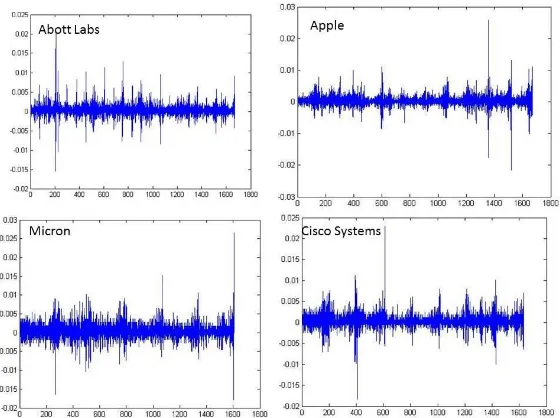
To check for the empirical relevance of our model, we considered data from the recent

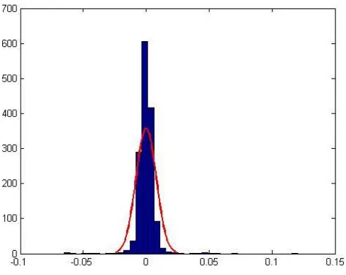
and Fig. 1). Returns are clearly non-Gaussian. Fig. 2 shows the histogram of the Apple stock and

its poor Gaussian fit.

Table 1. The stock returns for the period covering the mini flash crashes are not normally distributed.

Stock Time period Lilliefors test Excess kurtosis Reject normality?

Abott Labs April, 29 2011 – May, 31 2011 0.001 15.36 Yes

Apple March, 16 2012 − March, 30 2012 0.001 24.33 Yes

Cisco Systems July, 20 2011 − July, 29 2011 0.001 24.31 Yes

Core Molding August, 19 2011 − August, 31 2011 0.001 9.69 Yes

Note: The critical values were computed using Monte Carlo simulation for sample sizes less than 1,000 and significance levels between 0.001 and 0.5. The result 0.5 means the data are generated by a Gaussian, and 0.001 means rejection of Gaussianity

Fig. 2. Apple’s return histogram and Gaussian fit

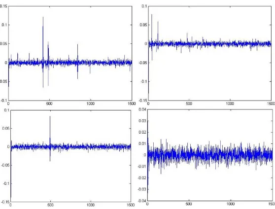
Fig. 3 shows the log-returns generated by our model for _i 1; an upper bound of

0.16

x  ; four groups of expectation targets (i4); and 25 percent of stop-loss agents. Fig. 4 shows the histogram. After comparing with the previous Figs. 1 and 2, one can see that the

model roughly replicates actual stock market behavior.

Fig. 4. The model return histogram and Gaussian fit; compare with Fig. 2

We are thus confident to proceed and explore some numerical implications of our model.

Table 2 shows selected simulation results using NetLogo

(http://modelingcommons.org/browse/one_model/3985#model_tabs_browse_procedures) for the

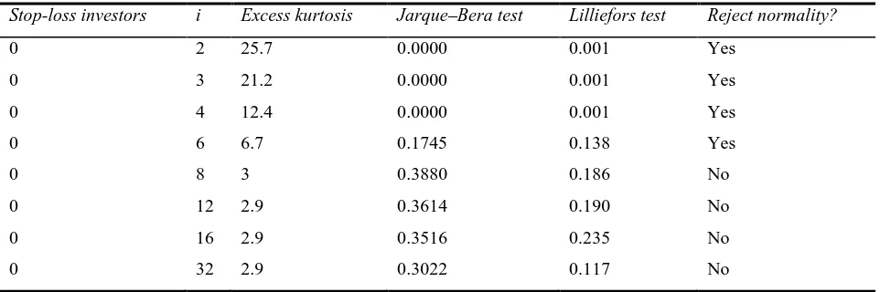
benchmark case where all 10,000 agents are disposition-effect investors. We first assume 1

and x 0.16. Excess kurtosis abates and the market becomes more Gaussian as we add more groups with distinct return targets (as we increase i). Thus, greater diversity of return targets

contributes to market efficiency, if Gaussianity can be translated into market efficiency [7].

Kaminski and Lo [4] proved stop-loss strategies cannot generate any excess profits if returns are

i.i.d., and the (weak) efficient market hypothesis assumes a white noise in the distribution of

returns. In our model, if we drop the disposition effect from the model, returns become Gaussian.

The very existence of disposition-effect investors makes it possible for stop-loss investors to

profit. In a non-Gaussian environment, which occurs when the disposition effect is considered,

Table 2. The model returns when all the agents are disposition-effect investors.

Stop-loss investors i Excess kurtosis Jarque–Bera test Lilliefors test Reject normality?

0 2 25.7 0.0000 0.001 Yes

0 3 21.2 0.0000 0.001 Yes

0 4 12.4 0.0000 0.001 Yes

0 6 6.7 0.1745 0.138 Yes

0 8 3 0.3880 0.186 No

0 12 2.9 0.3614 0.190 No

0 16 2.9 0.3516 0.235 No

0 32 2.9 0.3022 0.117 No

Table 3 shows the effect of the introduction of stop-loss agents who have the same x .

Now the agents cannot contribute to make the market more Gaussian. With i4, however, we cannot reject return normality. The presence of stop-loss agents reduces the importance of the

disposition effect in such a non-Gaussian environment. As observed, in Ref. [4] stop-loss rules

cannot stop losses for Gaussian returns, but are effective for non-Gaussian ones. Our model

confirms this. Starting from an endowment, agents using the stop-loss rule profit constantly,

while others are subject to both gains and losses.

Table 3. The model returns after the introduction of stop-loss investors.

Stop-loss investors i Excess kurtosis Jarque–Bera test Lilliefors test Reject normality?

5 4 16 0.0000 0.0010 Yes

10 4 16 0.0000 0.0200 Yes

20 4 22 0.0000 0.0010 Yes

30 4 23 0.0000 0.0010 Yes

40 4 14 0.0000 0.0010 Yes

50 4 10 0.0000 0.0010 Yes

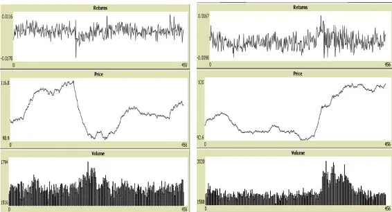
Our model recalculates the market sentiment index for each of the 50 periods. A

once-and-for-all negative shock of −20 to I can make the stock price dip, after 100 periods, from 116

Fig. 5. Effects of shocks coming from the market sentiment index I

Fig. 6 shows the effect of overconfident agents as _i increases. Considering 25 percent

of stop-loss investors and i4, as _i rises, both price and volume increase. As a result, overconfidence, which is accompanied by larger trade volume does not necessarily translate into

losses for the investors. This is because the volume increase is not due to the disposition-effect,

and the stop-loss agents are not affected by changes in _i.

Fig. 6. The effect of overconfidence as _i increases from 0.1 to 1 and then to 10

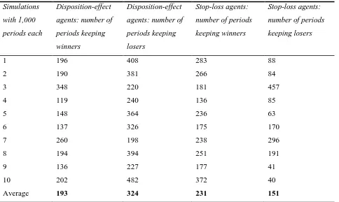
The 10 simulation results in Table 4 show that the two groups of agents behave in tandem.

The stop-loss agents keep winners 20 percent longer than the disposition-effect agents. And the

4. Conclusion

We set up a model of the stock market that considers agents subject to the disposition

effect and an offsetting stop-loss rule. The model can replicate actual return behavior considering

data from the recent mini flash crashes. We explore the consequences of altering key behavioral

parameters and show that differing return targets contribute to market efficiency; that a negative

shock to the market sentiment index causes the stock price to dip and trade volume to grow; and

that increasing overconfidence generates higher trade volume. More importantly, the presence of

stop-loss agents in a non-Gaussian environment offsets the disposition effect.

Table 4. Offsetting the disposition effect

Simulations

with 1,000

periods each

Disposition-effect

agents: number of

periods keeping

winners

Disposition-effect

agents: number of

periods keeping

losers

Stop-loss agents:

number of periods

keeping winners

Stop-loss agents:

number of periods

keeping losers

1 196 408 283 88

2 190 381 266 84

3 348 220 181 457

4 119 240 136 85

5 148 364 236 63

6 137 326 175 170

7 260 198 238 296

8 194 394 251 191

9 136 227 177 41

10 202 482 372 40

Average 193 324 231 151

Conflict of Interests

The author declares that there is no conflict of interests.

REFERENCES

[2] Kukacka, Jiri, and Jozef Barunik. "Behavioural breaks in the heterogeneous agent model: The impact of herding, overconfidence, and market sentiment." Physica A: Statistical Mechanics and its Applications 392.23 (2013): 5920-5938.

[3] Li, Yan, and Liyan Yang. "Prospect theory, the disposition effect, and asset prices." Journal of Financial Economics 107.3 (2013): 715-739.

[4] Kaminski, Kathryn M., and Andrew W. Lo. "When do stop-loss rules stop losses?." Journal of Financial Markets 18 (2014): 234-254.

[5] Tversky, Amos, and Daniel Kahneman. "Advances in prospect theory: Cumulative representation of uncertainty." Journal of Risk and uncertainty 5.4 (1992): 297-323.

[6] Barberis, Nicholas, and Wei Xiong. "What Drives the Disposition Effect? An Analysis of a Long‐Standing Preference‐Based Explanation." the Journal of Finance 64.2 (2009): 751-784.

[7] Suhadolnik, Nicolas, Jaqueson Galimberti, and Sergio Da Silva. "Robot traders can prevent extreme events in complex stock markets." Physica A: Statistical Mechanics and its Applications 389.22 (2010): 5182-5192. [8] Couzin, Iain D., et al. "Effective leadership and decision-making in animal groups on the move." Nature

433.7025 (2005): 513-516.

[9] Shiller, Robert J. "Measuring bubble expectations and investor confidence." The Journal of Psychology and Financial Markets 1.1 (2000): 49-60.