Framework for Continuous Improvement of Production Processes
Jevgeni Sahno
1, Eduard Shevtshenko
1, Tatjana Karaulova
1, Khadija Tahera
21Tallin University of Technology
Ehitajate tee 5, 19086, Tallinn, Estonia
E-mail. jevgeni.sahno@gmail.com, eduard.sevtsenko@ttu.ee, tatjana.karaulova@ttu.ee
2The Open University
Walton Hall, Milton Keynes, MK7 6AA, UK E-mail. k.tahera@open.ac.uk
http://dx.doi.org/10.5755/j01.ee.26.2.6969
This research introduces a new approach of using Six Sigma DMAIC (Define, Measure, Analyse, Improve, Control) methodology. This approach integrates various tools and methods into a single framework, which consists of five steps. In the Define step, problems and main Key Performance Indicators (KPIs) are identified. In the Measure step, the modified Failure Classifier (FC), i.e. DOE-NE-STD-1004-92 is applied, which enables to specify the types of failures for each operation during the production process. Also, Failure Mode and Effect Analysis (FMEA) is used to measure the weight of failures by calculating the Risk Priority Number (RPN) value. In order to indicate the quality level of process/product the Process/Product Sigma Performance Level (PSPL) is calculated based on the FMEA results. Using the RPN values from FMEA the variability of process by failures, operations and work centres are observed. In addition, costs of the components are calculated, which enable to measure the impact of failures on the final product cost. A new method of analysis is introduced, in which various charts created in the Measure step are compared. Analysis step facilitates the subsequent Improve and Control steps, where appropriate changes in the manufacturing process are implemented and sustained. The objective of the new framework is to perform continuous improvement of production processes in the way that enables engineers to discover the critical problems that have financial impact on the final product. This framework provides new ways of monitoring and eliminating failures for production processes continuous improvement, by focusing on the KPIs important for business success. In this paper, the background and the key concepts of Six Sigma are described and the proposed Six Sigma DMAIC framework is explained. The implementation of this framework is verified by computational experiment followed by conclusion section.
Keywords: Failure Classifier (FC), Failure Mode and Effect Analysis (FMEA), Process/Product Sigma Performance Level (PSPL), Failure Cost Calculation (FCC), Cost Weighted Factor for Risk Priority Number (CWFRPN).
Introduction
In order to be competitive and successful on the market place and satisfy customers, companies should continuously improve their production processes and product quality. The features of reliable and stable production process: less scrap, less rework, less the consumption of additional recourses, time and money.
From the literature review of the various sources that describe the scientific achievements made in the field of FMEA and Six Sigma, it can be summarised that the main goal of these methods is continuous improvement of business processes. Initially, researchers used these methods independently in order to achieve their goals. However, later, researchers started to combine these methods in order to achieve results that are more efficient.
Initially the Six Sigma methodology was developed for elimination of variability, and lean manufacturing for elimination of wastes in business processes (Womack et al., 1990; Womack & Jones, 1994). Later, these methodologies have been combined with DMAIC method for structural approach of problem solving. This combination later became known as Lean Six Sigma (Aon Management Consulting, 2003; Brook, 2010). There are many different
tools that are used in Lean Six Sigma, such as FMEA, Value Stream Mapping, Cause & Effect, Design of Experiments (DOE), SIPOC/COPIS, QFD/House of Quality and others (Brook, 2010). These methods are developed for various purposes, such as, measurement, analysis and improvement of business processes. But the most suitable Lean Six Sigma tool that intended to improve the reliability of business processes is FMEA (MacDermott et al., 1996). There are large amount of research papers where discussed common application of FMEA and Six Sigma for attainment of specific goals (Mekki, 2006; Krishna & Dangayach, 2007; Sarkar, 2007; Yang et al., 2010; Bhanumurthy, 2012; Chiarini, 2012). Based on comprehensive literature review results, it is possible to discover what achievements have not yet been done by combining these methodologies together:
Calculate Sigma performance level that shows the level of process or product quality based on the data from FMEA.
Calculate the financial impact of failure, in the process, on the final product cost using the data from FMEA.
and improve them. All these questions will be discussed further in the current paper.
The reason for selection of Six Sigma DMAIC methodology in current research, because today it is well-known methodology used in many companies around the world. However, every company can apply presented approach in another well-known methodology like PDCA, 8D or 4Q (Sahno & Shevtsenko, 2014).
Research Objectives and Scope
The objective of this research is to develop the framework for continuous improvement of reliability of production processes that allows improving KPIs - product Quality and Cost. This framework should integrate various quality improvement tools and methodologies. The new framework will be applied in rigorous Six Sigma DMAIC methodology that enables to define, measure, analyse improve and control problematic production process.
This framework helps engineers to find problematic operations and eliminate root causes of problems quickly and with less effort. The framework would play the role of a “dashboard” like in a cockpit, which allows monitoring the specified indicators such as Process/Product Sigma Performance Level (PSPL) and Cost Weighted Factor for RPN (CWFRPN). These subsequently influence Quality KPI
and Cost KPI in an up-to-date way due to the constantly renewed data from production floor, for example, data from Enterprise Resource Planning (ERP) system (Umble et al., 2003).
The framework is oriented towards the improvement of production processes in production floor, it is suitable for SMEs and can be applied in big enterprises, which have batch production.
Key Concepts Applied in the Research
This section provides the background of basic concepts and definitions that have been used in this research.
Key Performance Indicators (KPIs). KPI is a measure of performance; it is very useful for evaluating the current status of a company and for foreseeing the possible benefits of adopting an innovation in the system. KPIs are quantifiable measurements and depend on the particular company, which would evaluate those (Barchetti et al., 2011). Performance measurement is a fundamental principle of management and it is important because it identifies the gaps between current and desired performance, also provides indication of progress towards closing the gaps. Carefully selected KPIs identify precisely where to take action to improve performance (Weber et al., 2005).
Production Route (PR) card. It is a card that gives the detail of an operation to be performed in a production line. It is used to instruct the production people to take up the production work. The content and formats of the PR card can vary from a company to company. In general, it contains: an item and the number of quantities to be produced; production time; dimensions; any additional information that may be required by the production worker. PR card traces the route to be taken by a job during a production process (PR card 09.2013).
Failure Mode and Effect Analysis (FMEA). It is a systematic method of identifying and preventing product and process problems before they occurred. In recent years, companies are using FMEA to enhance the reliability and quality of their products and processes (Johnson 1998). The risk of a failure and its effects in FMEA are determined by three factors:
Severity (S) – the consequence of a failure that might occur during process.
Occurrence (O) – the probability or frequency of that failure occurring.
Detection (D) – failure being detected before the impact of the effect realized.
Every potential failure mode and cause is rated in these three factors on a scale ranging from 1 to 10. By multiplying these rating (See Equation 1), a Risk Priority Number (RPN) is generated. This RPN is used to determine the effect of a failure.
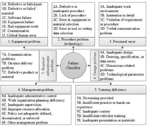
RPN = S × O × D (1) The RPN ranges from 1 to 1000 for each failure mode. It is used to rank the need for corrective actions to eliminate or reduce the potential cause of failures (MacDermott et al., 1996). All FMEAs are team based and the purpose of FMEA team is to bring a variety of perspectives and experience to the project (Stamatis, 2003). Failure Classifier (FC). Reliability engineering deals with an analysis of the causes of the faults in factories. In this paper a Failure Classifier (FC) is developed based on DOE-NE-STD-1004-92 standard, shown in Figure 1. There are seven major cause categories, and each has its subcategories. The basic goal of using this standard is to define the problems or causes that might occur for each operation during production process, in order to further correct them (DOE-NE-STD-1004-92, 09.2013). This standard was adapted and modified for the machinery enterprises (Karaulova et al., 2012).
Figure 1.Failure Classifier
(Stephens et al., 2007). Motorola was the first company who launched a Six Sigma project in the mid-1980s (Rancour et al., 2000). Since then, the applications of the Six Sigma methods allowed many organizations to sustain their competitive advantage by integrating their knowledge of the process with statistics, engineering, and project management (Anbari, 2002). It is a project-driven management approach intended to improve the products, services and processes of organizations by reducing defects. It is a business strategy that focuses on improving customer requirements understanding, business systems, productivity, and financial performance (Kwak et al., 2006; Desai et al., 2008). Six Sigma’s DMAIC method offers a thorough roadmap for analysis and diagnosis of problems; driven by powerful tools and techniques (Van Den Heuvel et al., 2006). The steps of the Six Sigma DMAIC are described in this section.
Define step is where a problem is identified and quantified in terms of the perceived result. The product and/or process to be improved are identified, resources for the improvement project are put in place and expectations for the improvement project are set. Measure step enables to understand the present condition of its work process before it attempts to identify where they can be improved. The critical to-quality characteristics are defined and the defects in the process/product developed through graphical analysis. All potential effects on failure modes are identified.
Analyse step adds statistical strength to problem analysis, identifies a problem´s root cause and determines how much of the total variation is.
Improve step aims to develop, select and implement the best solutions with controlled risks. The effect of the solutions that are then measured with the KPI developed during the Measure step.
Control step is intended to design and implement a change based on the results made the Improve step. This step involves monitoring the process to ensure it works according to the implemented changes, capture the estimated improvements and sustain performance (Watson, 2004).
From the statistical point of view, the term Six Sigma is defined as having less than 3,4 Defects Per Million Opportunities (DPMO) or a success rate of 99,9997 %, where sigma is a term used to represent the variation about the process average (Antony et al., 2002). If a company is operating at three sigma levels for quality control, this is interpreted as achieving a success rate of 93,32 % or 66807 DPMO. Therefore, the Six Sigma method is a very rigorous quality control concept, where many organizations still performs at three sigma levels (McClusky 2000). Today, to calculate DPMO, it is used the following Equation 2 (Seemer, 2010) and sigma performance scale table presented in Table 1, which enables to define Process/Product Sigma Performance Level on the basis of DPMO or process yield.
O U D
DPMO 1000000 (2)
where:
DPMO – product sigma performance level or DPMO level;
ΣD – sum of real defects occurred;
ΣU – sum of units produced/tested;
ΣO – sum of opportunities for defects per unit. It can take a long time for a company to produce a million of items, but it is not so important; this scale is just a projection of the number that would happen if a company will produce this amount. To define on what sigma performance level company operates, it can be identified the percentage of the Process Yield (PY) (see Equation 3) and defined the corresponding sigma level in the sigma scale table (Six Sigma, 15.01.2015).
100
O D O
PY (3) Table 1
Sigma performance scale table (Watson, 2004)
Sigma Performance Level
Defects per Million Opportunities (DPMO)
Process Yield
1,0 δ 670000 33 %
2,0 δ 308537 69,2 %
2,78 δ 100000 90 %
3,0 δ 66807 93,32 %
4,0 δ 6210 99,38 %
5,0 δ 233 99,9767 %
6,0 δ 3,4 99,99966 %
Six Sigma DMAIC framework
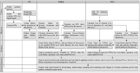
This section presents the new framework for continuous improvement of reliability of production process and KPIs. Proposed framework is presented in Figure 2 that shows the Quality-Cost (QC) framework in Six Sigma DMAIC structure. The details of the framework is explained below.
Define. The problematic process should be defined and the required KPI metric(s) for continuous improvement must be evaluated and indicated.
Measure. In Measure step, three different tools/methods are applied: 1) Failure Classifier (FC), where failures are assigned for every problematic operation in the process; 2) Failure Mode and Effect Analysis (FMEA), where every failure type weighted by Severity, Occurrence and Detection rating, calculated RPN value (in this research it will be named RPNReal) and PSPL (Sahno et al.,
2013); 3) Failure Cost calculation (FCC), where the costs are calculated at the Bill of Material (BOM) level and financial impact of failure on final product. The applications of these tools/methods are described below.
Measure in FC. During the production process, an operation may have failure; therefore the Failure Cause/Group should be assigned to the problematic operation from the FC. This step is the basis for the next two steps in FMEA and FCC.
Measure in FMEA. One of the purposes of the FMEA is to assess the risks of the production processes that influence on product quality. Therefore, the purpose of the FMEA in this research is to monitor the product Quality KPI by reducing RPNReal value of failures or eliminating
them in the production process.
production floor. As for Severity and Detection ratings, they will be assessed in a team as usually using the FMEA
rank tables. The techniques assessing these rating are described below.
Figure 2. Framework for continuous improvement of production processes inSix Sigma DMAIC structure
Severity assessment: The goal of this rating is to assess how critical the effect of a potential failure mode is on the overall system or process. In some cases, it is clear from past experiences. In current research the rating of Severity is defined from the Severity ranks table and it is based on the knowledge and experience of the team members (MacDermott et al., 1996).
Occurrence assessment: This rating is intended on assessment of failure frequency in production process. Occurrence is assessed according to the statistical data collected from production floor for the specified period of time (for instance, for one month). Below is presented Equation 4 that shows the way of calculation of Index of Occurrence (IO).
% 100
Q Q O
P S
I (4) where:
ΣSQ – scrap (non-qualified components/products)
quantity occurred for the specified period;
ΣPQ – produced product quantity for the specified
period.
When the percent value for the Occurrence is calculated, it should be defined Occurrence rating from Occurrence ranks table (MacDermott et al., 1996). For example, if there was checked 100 units and defined 10 scrap units, then the rating may equal to 10 points.
Detection assessment: The assessment of Detection is related to the performance of measurement tool that should check the required parameters in product and detect failures, before a product goes to a customer. In current research the rating of Detection is defined from the Detection ranks table and it is based on the knowledge and
experience of the team members (MacDermott et al., 1996).
RPN real (RPNReal) value per failure calculation: By
multiplying the three factors (S×O×D), the RPNReal value is
calculated for each failure.
RPN real (RPNReal) value per operation, work centre,
BOM level and process calculation: To calculate the sum of RPNReal value per operation, work centre, BOM level and
process, all RPNReal values per failure should be summed up.
Theoretical RPN (RPNTheoretical) value calculation: The
maximum RPNReal value for Severity, Occurrence and
Detection rating may equal to 10 points, subsequently the maximum RPNTheoretical value for the failure can be 1000
points.
Theoretical RPN (RPNTheoretical) per process
calculation: To calculate the sum of RPNTheoretical value for
the process/product, it should be counted the number of failures in the production process and multiplied by 1000 points. This RPNTheoretical value shows the scope of the
process or the maximum RPNReal value, which can be
reached or to be failed.
RPNReal percent calculation: To calculate the PSPL
(which is described further), it should be calculated first RPNReal percent value using the Equation 5.
% 100
% Re
Re
l Theoretica
al al
RPN RPN
RPN (5)
where:
ΣRPNReal – sum of real RPN for a particular product,
ΣRPNTheoretical – sum of theoretical RPN for a particular
Process Yield (PY) calculation: Having calculated RPNReal percent, now it can be calculated Process Yield
(PY), using the Equation 6.
PY = 100% –RPNReal% (6)
where:
100 % – maximum percent value of ΣRPNTheoretical
Process/Product Sigma Performance Level (PSPL) calculation: The PSPL in this research shows the level of process/product quality that can be calculated using the RPNReal per failure, operation, work centre, BOM level and
common process, and RPNTheoretical values calculated in
previous steps. Having calculated PY and according to the sigma performance scale in Table 1, the PSPL can be defined.
Measure in FCC. The purposes of the FCC approach in this research is to calculate Cost Weighted Factor for RPN (CWFRPN) that shows failure financial impact (calculated in
FMEA) on final product. In current research this factor should be reduced by improving or eliminating the RPNReal
values of failures in FMEA that influence on product Cost KPI. To calculate CWFRPN for failure, operation and work
centre it should be firstly calculated Cost of Material and Operation (CMO) and to calculate CWFRPN for BOM level,
the Cost of BOM Level (CBOML) should be calculated too.
Cost of Material and Operation (CMO) calculation: To
calculate CMO, the Cost of Material (CM) and Cost of
Operation (CO) should be summed. See Equation 7.
CMO = CM + CO (7)
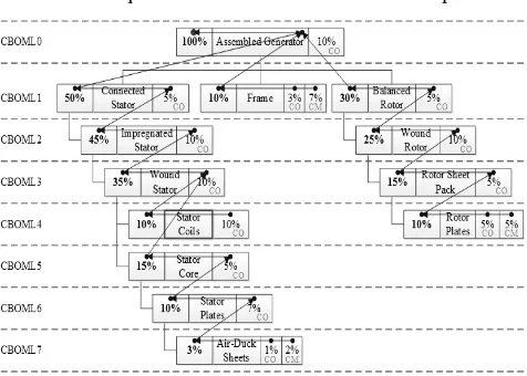
Cost of BOM Level (CBOML) calculation: In Figure 3, an example of product BOM structure is presented that consists of BOM levels and which contain other sub-levels and subsequent lower levels. The total cost of product equals to 100 % and this is the cost of BOM level zero – CBOML0. The cost of CBOML0 equals to the sum of operation
cost (∑CO0) and sum of material cost (∑CM1) from BOM
level 1 (CBOML1). Further, the cost of CBOML1 equals to the
sum of operation cost (∑CO1) and sum of material cost
(∑CM2) from BOM level 2 (CBOML1) and so forth until the
lower level of a product. To calculate the CBOMLN, it is
proposed to use the Equation 8. yi C yi C
C O
m
y n
i M BOMLN
1 1
(8)
where:
CBOMLn – cost of Bill Of Materials (BOM) of level n,
y = 1 ÷ m – number of BOM levels;
i = 1 ÷ n – number of components in BOM level; CMn – material cost of BOM level n;
COn – operation cost of BOM level n.
Figure 3. Product BOM structure with levels
Cost Weighted Factor of RPN (CWFRPN) calculation:
Based on the previous step, where CMO and CBOMLN was
calculated, now, it should be calculated CWFRPN per every
failure, operation, work centre and BOM level that shows the financial impact on final product. To calculate CWFRPNFOW per failure, operation, work centre the Equation
9 should be applied. To calculate CWFRPNBOMLN per BOM
level, the Equation 10 should be applied.
al
BOML MO
RPNFOW RPN
C C
CWF Re
0
(9)
al
BOML BOMLN
RPNBOMLN RPN
C C
CWF Re
0
(10) where:
CWFRPNFOW – CWF of RPN per failure, operation and
work centre,
CWFRPNBOMLN – CWF of RPN per BOM level N,
CMO – Cost Of Material and Operation,
CBOMLn – Cost of Bill Of Materials (BOM) of level n,
CBOML0 – upper BOM level that equals to 100% of
product cost,
∑RPNReal – sum of real RPN per failure, operation,
work centre and BOM level.
Figure 4. Production process structure for continuous improvement
Figure 4 shows the summary of Measure step where shown the new framework process that depicts the inputs of product production process and the failures that can occur. For example, a product contains components and
values in FMEA. Further the PSPL in FMEA and CWFRPN
in FCC calculated that influence on Quality and Cost KPIs. Analyse. The outcome of the Measure step enables to perform the analysis of production process/product and general production system in a different way for FMEA, and FCC phase, as described below.
Analyse in FMEA and FCC. Based on the received results in FMEA and FCC from Measure step, it should be built Chart for CWFRPN and Pareto Chart and made their
observation and comparison.
Chart for CWFRPN, CMO and RPNReal creation: This
chart should be built for an operation using CWFRPN and
CMO from FCC and RPNReal value from FMEA. This chart
visually should show which operations in the process/product have high RPNReal value, CMO and CWFRPN
comparing with other operations.
Pareto Chart creation: This chart should be built based on the calculated RPNReal values from FMEA and CWFRPN
from FCC, which indicates the most critical failures in production process. Further, these charts can be compared as follows:
It indicates that the failures of these charts are located in different sequence. The Pareto chart based on RPNReal
from FMEA shows failure sequence that are influence on Quality KPI. The Pareto chart based on CWFRPN from FCC
shows failure sequence that influence on Cost KPI. Comparing these charts, an engineer can make decision on which KPI is more important for some specified product type or for general production system or for some customer.
Analyse in FMEA. Using RPNReal values from FMEA,
it can be observed the process variability of work centres, operations and failures in the following way:
Work Centre: It should be selected specific work centre, which shows what operations and failures it has, it shows an average RPNReal value for specific work centre
and in what BOM level and product type it used.
Operation: A specific operation should be selected, that can show what failure types this operation has and in what work centre, BOM level and product type it is used. In addition, it can be selected for example, some specific operation in the process and calculated an average RPNReal
value, or selected all existing operations and defined most problematic operation with high RPNReal value.
Failure Group and/or Failure Cause: Failure Causes (sub-groups) should be grouped according to their main Failure Group. Further, it can be possible to see the specific failure variability by RPNReal value it has. In addition, it can
be observed in what operation, work centre, BOM level of the product that specific failure exists. In addition, an average RPNReal value of the failure for the process can be
calculated.
Analyse in FCC. The analysis in FCC should be explained using the following example. A BOM level has 10% of cost of final product and it has high RPNReal values
and at the same time there is another BOM level, which has 20% of cost of final product and it has same RPNRealvalues
or may be even lower, then, there should be made a decision for BOM level that has higher cost. In other words, the CWFRPN indicates the cost weight of failures,
operations and BOM levels of final product. This kind of cost weighted factor assessment allows engineers to pay attention on more important problems, which have
financial impact on final product. This approach allows decreasing the number of scrap, as a result it enables to save money and increase company revenue.
The above presented example may have exceptions. For instance, if a cost of some BOM level is 10 % of final product cost and it has high RPNReal values, but it does not
influence on entire product quality, e.g. a scrap component can be replaced or demounted from design point of view, then, in this case, the financial impact will be low. Another example, if a cost of BOM level is 10 % of final product cost and it has low RPNReal values, but it can influence on
entire product quality e.g. the scrap component cannot be replaced or demounted from the final product, as a result, an entire product may go to scrap, so the financial impact will be high. In this case, improvements should be made for BOM level, which has high financial impact on product.
Improve. Perform corrective actions based on the results from previous steps (measure, analyse): generate various potential solutions and select the best one, assess the effect of the solution (identify what KPI is more important for the particular product or for general production system or for customer) and implement the solution (reduce the RPNReal value for the harmful failure in
operation or eliminate them completely). The more reliable production process, the less process variability, the less number of defects, failures or RPNReal values in the process,
therefore, less product scrap and higher product Quality KPI. Subsequently, less product financial losses that in turn the higher Cost KPI. In case the improvement requires financial investment, it is necessary to calculate how soon the investment starts to pay off for itself (when the break-even point starts) (Badiru, 2005).
When the corrective actions applied, an engineer should follow them by performing “mini DMAIC” process, as follows:
Define the object of study that is something that has been corrected or improved.
Measure the improved process by assigning failures from FC and assessing RPNReal in FMEA.
Analyse processes and decide where and what corrective actions are necessary to carry out.
Improve process (if needed).
Control made improvements in daily processes, if the process requires to repeat an improvement, then repeat the "mini DMAIC" process again until the changes are satisfy.
Control. Ensure that the implemented solution is working by applying "mini DMAIC" process. If proposed changes are satisfying and not require any more corrective actions, then proceed to the improvements with other processes. Document, apply, sustain and monitor made improvements in real processes of everyday production.
This framework enables to decrease the number of defects/failures in the process, thus decreasing their RPNReal
value that in turn increases such indicators as Process/Product Sigma Performance Level (PSPL) and Cost Weighted Factor of RPN (CWFRPN) that influences on
Computational Experiment
In this research a computational experiment of the new framework for continuous improvement of production processes is checked with the production process related data. The computational experiment was made on a “Wind Power Generator A” product that is used in windmills for generation of energy. This product - assembly consists of some sub-assemblies that is presented in Figure 5 in the form of BOM structure.
Define. One of the main tasks of computational experiment in DMAIC is to identify problematic process and the main KPIs that should be continuously improved.
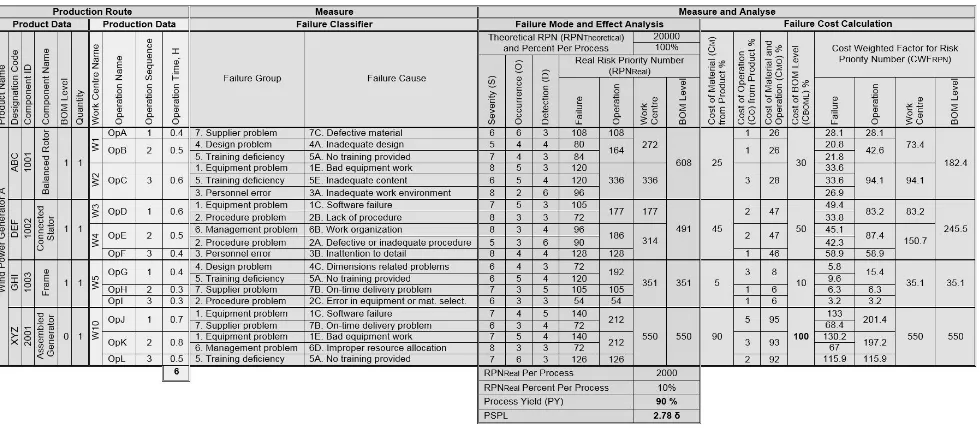
Process: The problematic process is displayed in the form of PR card with “Wind Power Generator A” product. The PR consists of two parts (see Figure 6): Product Data which contains product name to be produced, BOM levels of product, component ID and name, and quantity to be produced; Production Data which contains work centre name, where component to be processed, operations name, its sequence and operation time.
KPI: Today, to find out what KPIs are important for the customer, companies use survey techniques and questionnaires that enable to define them. In most cases, companies and customers calculate KPI metrics using its own calculations, for example based on received reclamations from production floor or customer. Taking into account the considerable complexity of the manufacturing sector, this research focused on two KPIs – product Quality and Cost.
Quality metric is a calculation of the amount of quality delivered units versus the amount of non-quality units. For instance: Company received 10 units. The order has 2 defect units. The Quality metric for this order is 80 %. Calculation: Number of quality units received / Total number of ordered units (8/10 = 80 %).
Cost metric is very important for any company that wants to increase their revenue, therefore the goal in this research is to increase company revenue by means of improving production processes reliability and Quality that in turn directly influence on Cost KPI.
The main KPI metrics have been identified and evaluated. Further it is presented new framework application with production related data that explains how process indicators which influence on KPIs can be calculated and improved.
Measure.In Measure step different tools/methods (FC, FMEA and FCC) are discussed.
Measure in FC. It is defined Failure Cause and Failure Group in FC for each operation during the production process (see Figure 6).
Measure in FMEA. In FMEA every failure assessed by Severity, Occurrence and Detection rating, which gives the RPNReal value. This value calculated for every failure,
operation, BOM level and process or product.
Severity assessment: Severity rating is defined according to the Severity scale that indicates the effect of a failure; it is based on the knowledge and experience of the team members (MacDermott, 1996).
Occurrence assessment: This rating intended on assessment of failure frequency in production process and in this computational experiment applied the following
example; the production line passed 500 units of a component during one month on operation “OpA” in work centre “W1”. From 500 units, there is 1 unit that has failure cause occurred – “7C. Defective material” that is in failure group – “7. Supplier problem”. To define Occurrence rating, the Index of Occurrence (IO) should be calculated
firstly using Equation 4 that shows that there are 0,2 % of failures each month. Then using this index, the Occurrence rating can be defined using the Occurrence rating table (MacDermott et al., 1996) which shows that 1 scrap in 500 units equals to 6 points of Occurrence rating – moderate.
% 2 , 0 % 100 500
1
O
I
Detection assessment: The purpose of this rating is to detect the failure before it happens on customer side. Before start failure detection, it should be beforehand specified parameters of the product that should be checked. The specified parameters of these units should be checked according to the customer needs. Before testing an item, it should be beforehand defined parameters, which customer needs to be tested, and if there are flaws, they should be defined and eliminated. If the failure was defined in further production stages or by customer on his side, the Detection value will increase (MacDermott, 1996).
RPN real (RPNReal) value per failure calculation: By
multiplying the three factors (S×O×D), the RPNReal value is
calculated for each failure (Figure 6).
RPN real (RPNReal) value per operation, work centre,
BOM level and process calculation: The sum of RPNReal
value was calculated by summing up all RPNReal values per
failure. For example 164 points per operation “OpB”; 272 points per work centre “W1”; 608 points per BOM level “1”; 2000 points per process (Figure 6).
Theoretical RPN (RPNTheoretical) per process
calculation: To calculate the RPNTheoretical per process it
should be counted the number of failures occurred in the process and multiplied by RPNTheoretical per failure (1000
points). Figure 6 shows the process of three assemblies or BOM level - “1” (Balanced Rotor, Connected Stator and Frame) and Assembled Generator or BOM level - “0” – which are processed in work centres. These work centres have 12 operations with 20 failures occurred. As the RPNTheoretical value for every failure is 1000 points
(10x10x10) and there found 20 failures in the process, the sum of RPNTheoretical value per process for the “Wind Power
Generator A” equals to 20000 points (20x1000). This value used to define the scope of the common production process that equals to 100 %.
RPNReal percent calculation: After calculating the sum
of RPNReal (2000 points) and RPNTheoretical (20000 points)
value for the process or product, now these values can be used to calculate RPNReal percent per process using the
Equation 5.
% 10 % 100 20000
2000 %
Real
RPN
Process Yield (PY) calculation: According to the above calculations, the RPNReal per process equals to 2000 points
that makes 10 % from RPNTheoretical value of 20000 points.
As the RPNReal equals to 10%, then the PY can be
calculated using the Equation 6, extracting the RPNReal per
PY = 100 % - 10 % = 90 %
Process/Product Sigma Performance Level (PSPL) calculation: As the PY equals to 90% that shows, according to the sigma performance scale in Table 1, the PSPL for the current process or product equals to 2,78 δ.
If the company produces 5 products and every product has its own PSPL, an average PSPL for all products can be calculated in the following way: the calculated PSPLs should be summed up and divided into 5 products. As the result, the average PSPL is 2,8 δ.
PSPLAverage = 2,78 + 2,9 + 2,7 + 3 + 2,6 ≈ 2,8 δ
Measure in FCC. The FCC phase in this research divided into two parts: in the first part calculated CMO and
CBOML that is the basis for the CWFRPN calculation.
Cost of Material and Operation (CMO) calculation: To
calculate CMO, the CM (25 %) and CO (1 %) should be
summed (Figure 6) using Equation 7. It shows that the cost of material of “Balanced Rotor” and operation “OpA” equals to 26 %. Further, this value used to calculate CWFRPN per failure, operation and work centre.
CMO = 25 + 1 = 26 %
Cost of BOM Level (CBOML) calculation: In Figure 5
presented an example of product BOM structure. From the right side of each component, assembly and final product defined value-added operation cost (CO) (in per cent value).
For instance, the CO of Assembled Generator is 10% from
the final product cost, it means the assembled together Connected Stator, Frame and Balanced Rotor costs to 10% of final product. From the left side defined the value-added material cost (CM) (in per cent value), which includes the
cost of BOM of lower level (CBOMLN-1), because the lower
level BOM is the material/component (that already has cost) for the upper BOM level. The Equation 8 and values from Figure 5 is used to calculate the cost of CBOML1
(Connected Stator) and CBOML0 (Assembled Generator).
Cost Weighted Factor for RPN (CWFRPN) calculation:
To calculate the financial impact of failure, operation and work centre on final product the Equation 9 should be used. Below is presented the example for failure cause - 7.C Defective Material; operation - OpA; and work centre - W2.
Failure Cause: 7.C Defective Material
1 . 28 108 100
26
RPNFOW CWF Operation: OpA 6 . 42 ) 84 80 ( 100
26
RPNFOW
CWF
Work Centre: W2
1 . 94 ) 96 120 120 ( 100
28
RPNFOW
CWF
Same approach should be applied for every failure, operation and work centre in the process.
The similar approach should be applied for every BOM level in the process using the Equation 10.
BOML1: Balanced Rotor
4 . 182 ) 96 120 84 80 108 ( 100
30
RPNBOML
CWF
BOML1: Connected Stator
5 . 245 ) 128 90 96 72 105 ( 100
50
RPNBOML
CWF
CBOML1: Cost of Connected Stator = Connected Stator (CO1) + Impregnated Stator (CBOML2)
CBOML1 = ΣCO1 + ΣCBOML2
CBOML1 = 5% + 45% = 50%
CBOML0: Cost of Assembled Generator = Assembled Generator (CO0) + (Connected Stator (CBOML1) + Frame
(CBOML1) + Balanced Rotor (CBOML1))
CBOML0 = ΣCO0 + ΣCBOML1
CBOML0 = 10% + (50% + 10% + 30%) = 100%
Same approach should be applied for remained BOM levels and components until the lower level of the product.
Figure 5. Assembled Generator BOM structure
Analyse.The results from the Measure step enable to create various charts and diagrams, and perform the analysis of the data from FMEA and FCC phases.
Analyse in FMEA and FCC. Based on the calculated data in FMEA and FCC, from the Measure step, it is created various charts that allow analyse these results. The Cost Weighted Chart for CWFRPN and Pareto charts are
built and their comparison made.
Chart for CWFRPN, CMO and RPNReal creation: Figure 7
presents Cost Weighted Chart for RPNReal per operation
from FMEA, for CWFRPN and CM and CO from FCC. This
chart visually shows which operations have high RPNReal
value (quality), CWFRPN and CMO (cost) impact on final
product (for example these are operations “OpJ” and “OpK”). The chart shows that these operations are critical from all point of views (quality and cost) and they have priority for improvement comparing with others, for example, visually it can be noticed that operation “OpI” has low RPNReal value, material/component cost and low
CWFRPN. Other words it does not have high impact on
Figure 6. Integrated report of PR card, FC, FMEA and FCC
Figure 7. Chart for RPNReal, CMO and CWFRPN per operation
Pareto chart creation for RPNReal: Based on the
calculated RPNReal values from FMEA (Figure 6), it is
created Pareto chart per failure that also shows in what operation it happened. The chart presented in Figure 8 indicates the most critical failures in production process from product quality point of view. Using this chart, an engineer can define what failures should be eliminated or at least where RPNReal values should be decreased in order to
improve PSPL that influence on Quality KPI.
Figure 8. Pareto chart for RPNReal of failure per operation
Pareto chart creation for CWFRPN: Based on the
calculated CWFRPN values from FCC (Figure 6), it is
created Pareto chart for per failure that also shows in what operation it happened (similar as for RPNReal presented in
Figure 8). The chart presented in Figure 9 indicates the most critical failures in the process from financial point of view. Using this chart, an engineer can define what failures should be decreased or eliminated to improve product CWFRPN that influence on Cost KPI.
Figure 9. Pareto chart for CWFRPN of failure per operation
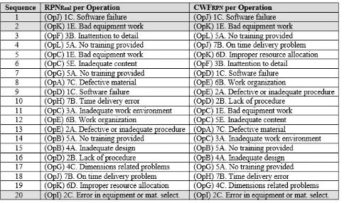
Comparing these two charts, it shows that the failures have different sequence. For example, the sequence of failures in Pareto chart for RPNReal in FMEA is different
from the sequence of failures in Pareto chart for CWFRPNin
FCC. Figure 10 presents failure sequence difference which shows that the sequence of only three failures/operations was not changed (1, 2, 20), all other failures are in different sequence. It is operations (“OpJ”, “OpK” and “OpI”) that has been already mentioned in Figure 7. It shows that operations “OpJ” and “OpK” are very critical from all quality and cost point of view and the operation “OpI” has low importance. Comparing these results, an engineer, for instance, can make decision that it is more essential for the current process to improve first two operations that influence on PSPL and CWFRPN indicators and
Figure 10. Summary of failure sequence from Pareto charts
Analyse in FMEA. By applying the RPNReal values from
FMEA it can be observed the process variability of work centres, operations and failures, identified minimum and maximum RPNReal value per failure, in addition it can be
calculated an average RPNReal value per general production
process. Every production process may consist of many different operations, which operate in a specified order; moreover, these operations can be reused in same production process. In addition, some specified operation may have different or even same failure cause and same or different RPNReal value in same production process and/or
in general production system. Other words, the variability may be huge. This kind of process analysis allows better understand what work centres, operations and failures are critical for the general production system. Engineer can identify the most harmful failures with high RPNReal value
and improve or eliminate it. Similar analysis can be done not only for general production system, but also for some specified product type.
Analyse in FCC. After calculating CWFRPN for both
BOM levels (Connected Stator and Balanced Rotor) in Measure step, it can be done the following summary using the data from Figure 6. The CWFRPN value for Connected
Stator is higher than CWFRPN value for Balanced Rotor,
despite of the fact that the Balanced Rotor has more failures and higher RPNReal value per BOM level in FMEA
than Connected Stator. It means that the improvements should be done on Connected Stator that has high financial impact on final product.
Improve. Based on the results from the first two steps, an engineer can develop improvement program that enables to decrease production process variability, number of defects or failures and improve production processes reliability. Below is presented example of corrective actions for every KPI.
In order to improve Quality KPI, it is first necessary to determine on what PSPL process operates and which failures are most harmful to the production process (using RPNReal values), i.e. determine what failures have a
negative impact on the quality of the semi-products as well as on the final product. The Figure 8 shows that the most harmful failures (according to the Pareto law 80/20) are: “(OpJ) 1C. Software failure”, “(OpK) 1E. Bad equipment work” and “(OpF) 3B. Inattention to detail”. These failures related to the “Equipment problem” and “Personnel error” failure group. From here can be made summary, in order to reduce the RPNReal values of these failures or eliminate
them completely and increase PSPL that influence on Quality KPI, it is necessary to take corrective actions. For example, provide to employee required training how to operate machine, create simple and clear instruction guide and during the training period provide more experienced operator as the mentor who can help acquire needed experience.
The same approach should be carried out for the Cost KPI. It is necessary to determine which failures are most harmful from the financial point of view in the production process (using CWFRPN values). Figure 9 shows that the
most harmful failures are: “(OpJ) 1C. Software failure”, “(OpK) 1E. Bad equipment work” and “(OpL) 5A. No training provided”. These failures related to the “Equipment problem” and “Training deficiency” failure group. As in the previous case, in order to improve Cost KPI, it is necessary firstly reduce the RPNReal values of the
failures or eliminate them completely that influence on high CWFRPN values. In that case, as in previous example,
there should be provided to employee required training how to operate machine, create simple and clear instruction guide and during the training period provide more experienced operator as the mentor who can help acquire needed experience.
From the two examples above, it can be done the following summary that the cause of poor product quality and financial losses is the lack of operator knowledge and experience. In that case, in order to increase these KPIs, company management should provide to the operators required trainings that increase their competence.
Control. The purpose of the Control step is to document and sustain made improvements and monitor implemented solution in daily production process. Check made improvements and apply “mini DMAIC” process if needed. Perform continuous improvements for the improved process. If the implemented corrective actions satisfy, then continuous improvement for other problem processes should be proceeding.
Conclusion
In this paper a new framework was demonstrated for continuous improvement of production processes using rigorous Six Sigma DMAIC methodology. In the Define step, the problem and main KPIs for improvement are identified. In the Measure step, the modified Failure Classifier (FC) standard, i.e. DOE-NE-STD-1004-92 was applied, which enabled to specify the types of failures for each operation during the production process. In addition, the Failure Mode and Effect Analysis (FMEA) is applied to assess the weight of the each failure by Severity, Occurrence and Detection rating and then calculated the RPNReal value. Based on the FMEA results, the PSPL was
calculated that indicated the general level of quality for the process/product that influence on Quality KPI. Using the RPNReal values from FMEA the variability of the process by
failures, operations work centres and BOM level was observed. In addition, the costs of the components and/or BOM level was calculated in FCC, in order to further define the financial impact of failure (CWFRPN) on final
This framework enables an engineer to perform daily monitoring of production processes (based on data for the previous day); determine what failure is the most harmful in the process from product quality and cost and point of
view; perform continuous improvement of production processes and their indicators that affect the KPIs, this in turn helps to improve customer satisfaction and financial performance of the company.
Acknowledgement
Hereby we would like to thank the Estonian Ministry of Education and Research for Grant ETF9460 which supports the research.
References
Anbari, F. T. (2002). Six sigma method and its applications in project management. In Proceedings of the Project Management Institute Annual Seminars and Symposium [CD], San Antonio, Texas. Oct (Vol. 3, No. 10). http://dx.doi.org/10. 1108/13683040210451679
Antony, J., & Banuelas, R. (2002). Key ingredients for the effective implementation of Six Sigma program. Measuring Business Excellence, 6(4), 20–27.
Aon Management Consulting. (2003). Lean Six Sigma. Leadership Report.
Badiru, A. B. (2005). Handbook of industrial and systems engineering, CRC Press. http://dx.doi.org/10.1201/9781420038347 Barchetti, U., Bucciero, A., Guido, A. L., Mainetti, L., & Patrono, L. (2011). Supply Chain Management and Automatic
Identification Management convergence: Experiences in the Pharmaceutical Scenario. Supply Chain Coordination and Management. Vienna: IN-TECH Education and Publishing.
Bhanumurthy, M. V. (2012). Profitability through lean Six Sigma: Save energy - Save environment. AIChE Annual Meeting, Conference Proceedings.
Brook, Q. (2010). Lean Six Sigma and Minitab. The Complete Toolbox Guide For All Lean Six Sigma Practitioners.
Chiarini, A. (2012). Risk management and cost reduction of cancer drugs using Lean Six Sigma tools. Leadership in Health Services, 25(4), 318–330. http://dx.doi.org/10.1108/17511871211268982
Desai, T. N., & Shrivastava, R. L. (2008, October). Six Sigma–a new direction to quality and productivity management. In Proceedings of the World Congress on Engineering and Computer Science, San Francisco, CA. Elsevier.
DOE-NE-STD-1004-92. (1992). Root Cause Analysis Guidance Document, US http://www.everyspec.com/DOE/DOE+ PUBS/DOE_NE_STD_1004_92_262 (11.2012).
Hennig-Thurau, T., & Klee, A. (1997). The impact of customer satisfaction and relationship quality on customer retention: A critical reassessment and model development. Psychology & Marketing, 14(8), 737–764. http://dx.doi.org/10.1002/ (SICI)1520-6793(199712)14:8<737::AID-MAR2>3.0.CO;2-F
Johnson, S. K. (1998). Combining QFD and FMEA to optimize performance. In Annual Quality Congress Proceedings-American Society For Quality Control, 564–575.
Karaulova, T., Kostina, M., & Sahno, J. (2012). Framework of reliability estimation for manufacturing processes. Mechanics, 18(6), 713–720.
Kostina, M., Karaulova, T., Sahno, J., & Maleki, M. (2012). Reliability estimation for manufacturing processes. Journal of Achievements in Materials and Manufacturing Engineering, 51(1), 7–13.
Krishna, R., & Dangayach, G. S. (2007). Six Sigma implementation at an auto component manufacturing plant: a case study. International Journal of Six Sigma and Competitive Advantage. 3(3), 282–302. http://dx.doi.org/10.1504/ IJSSCA.2007.015070
Kwak, Y. H., & Anbari, F. T. (2006). Benefits, obstacles, and future of six sigma approach. Technovation, 26(5), 708–715. http://dx.doi.org/10.1016/j.technovation.2004.10.003
MacDermott, R. E., Mikulak, R. J., & Beauregard, M. R. (1996). The basics of FMEA. Productivity Press.
McClusky, R. (2000). Six Sigma Special The rise, fall and revival of six sigma. Measuring Business Excellence, 4(2), 6–17. Mekki, K. S. (2006). Robust design failure mode and effects analysis in designing for Six Sigma. International Journal of
ProductDevelopment, 3(3), 292–304. http://dx.doi.org/10.1504/IJPD.2006.009895
Production Route Card, Available from: http://www.enotes.com/american-scholar/q-and-a/what-meant-by-job-card-route-card-used-production-99397, Accessed: 09.2013.
Rancour, T. and McCracken, M. (2000). Applying six sigma methods for breakthrough safety performance. American Society of Safety Engineers, 31–4.
Sahno, J., Sevtsenko, E., & Karaulova, T. (2013). Knowledge Management Framework for Six Sigma Performance Level Assessment. In Advances in Information Systems and Technologies. Springer Berlin Heidelberg, 255–267. http://dx.doi.org/10.1007/978-3-642-36981-0_25
Sahno, J., & Shevtshenko, E. (2014). Quality Improvement Methodologies for Continuous Improvement of Production Processes and Product Quality and Their Evolution. 9th International DAAAM Baltic Conference Industrial Engineering, 181–186. Sarkar, B. N. (2007). Designing sustainable strategies for continuous improvement deployment programme: lessons from a steel
plant in India. International Journal of Six Sigma and Competitive Advantage, 3(4), 352–376. http://dx.doi.org/10.15 04/IJSSCA.2007.017177
Seemer, R.H. (2010). Defects Per Million Opportunities (DPMO).
Six Sigma, Available from: http://www.isixsigma.com/new-to-six-sigma/sigma-level/how-calculate-process-sigma, Accessed: 01.2015.
Stamatis, D. H. (2003). Failure mode and effect analysis: FMEA from theory to execution. Asq Press.
Stephens, J. S., & McDonald Jr, C. L. (2007). Lean Six Sigma. The Journal of Organizational Leadership and business. Retrieved November, 24, 2010.
Umble, E. J., Haft, R. R., & Umble, M. M. (2003). Enterprise resource planning: Implementation procedures and critical success factors. European journal of operational research, 146(2), 241–257. http://dx.doi.org/10.1016/S0377-2217(02)00547-7 Van Den Heuvel, Does, R. J., & De Koning, H. (2006). Lean Six Sigma in a hospital. International Journal of Six Sigma and
Competitive Advantage, 2(4), 377–388. http://dx.doi.org/10.1504/IJSSCA.2006.011566
Watson G. H. (2004). Six Sigma for Business Leaders, First Edition, Business Systems Solutions, Inc. USA.
Weber, A., & Thomas, I. R. (2005). Key performance indicators. Measuring and Managing the Maintenance Function, Ivara Corporation, Burlington.
Womack, J. P., Jones, D. T., & Roos, D. (1990). The Machine that Changed the World: The Story of Lean Production HarperCollins Publishers, New York, USA.
Womack, J., & Jones, D. (1994). From lean production to the lean enterprise. Harvard Business Review, 72(2), 93–103.
Yang, M. S., Li, Y., Liu, Y., & Gao, X. Q. (2010). A Method for Problem Selection in the 6σ Definition Stage, Advanced Materials Research, 139, 1485–1489. http://dx.doi.org/10.4028/www.scientific.net/AMR.139-141.1485