AN
OVERVIEW
OF
DATA
STRUCTURES
AND
ALGORITHMS:
CASE
STUDY
OF
USE
IN
THE
VECTOR-SPACE
MODEL
AND
MINING
OF
FREQUENT
ITEMSETS
USING
THE
APRIORI
ALGORITHM
D. L. Nkweteyim
D
EPARTMENT OFC
OMPUTERS
CIENCE,
U
NIVERSITY OFB
UEA,
B
UEA,
CAMEROON
E-mail address:
[email protected]
ABSTRACT
In this paper, we review some commonly used data structures and algorithms. We then review two important problems: the creation of the vector-space model that is widely used in the design of information retrieval systems, and the mining of frequent itemsets using the apriori algorithm. We consider two variations of the apriori algorithm: the first is the classical algorithm which computes candidate k-itemsets by first joining frequent (k-1)-itemsets to themselves, and applying the apriori property to prune the generated candidate k-itemsets; the second avoids the join stage in the classical algorithm, and instead, generates candidate k-itemsets directly from rows of the transactions database, followed by application of the apriori property to prune each itemset so determined. Finally, we illustrate appropriate data structures and algorithms that when put together, provide efficient implementations of our solution to the problems mentioned.
Keywords: data structures, algorithms, vector-space model, frequent itemsets mining, apriori algorithm.
1. INTRODUCTION
An algorithm is a problem-solving method, implemented in a computer as a program. Most algorithms make use of data structures, which are essentially an organization of data in a form that is suitable for use by algorithms. The complexity of an algorithm is directly related to how much computing resources – principally processor time and/or memory requirements – are required to solve the problem. In problem-solving using a computer, a programmer chooses from a number of different algorithms which, when put together following a particular logic, lead to the solution of the problem.
Several algorithms are usually available to solve a problem, with some more complex than others. For small problems (that do not require much computing resources), it may not matter much which algorithms are chosen as the gain in time or the reduction in memory requirements for the most efficient algorithms might be negligible. Hence, the programmer may choose to use less efficient or effective algorithms for such problems, especially if they are relatively easy to implement.
For large, complex problems however, it is necessary to choose algorithms that manage space and/or time well, otherwise the running program may run out of memory required to do its computations, or the computations
may take too long to arrive at a solution. Carefully designed algorithms may reduce resource use by several orders of magnitude over poorly designed ones. And well-designed algorithms pay off far better than more sophisticated hardware (faster processors, larger memories). Hence, for large problems, it is much better to invest on efficient algorithms than on sophisticated hardware [1, 2].
In this paper, we review a number of widely used data structures and algorithms, highlighting their relative strengths and weaknesses. We then review two important processor- and memory-intensive problems, and the algorithms used to solve them. The problems addressed are: (1) the generation of document representations using the vector-space model that is widely used in information retrieval, and (2) generation of frequent itemsets in association rule mining using the apriori algorithm. The problem of generating frequent itemsets is considered from two perspectives: one is the classical apriori algorithm that has been widely studied [3–8] and involves an expensive join stage, and the other, a join-less apriori algorithm [9] that avoids the join stage in the classical algorithm. Finally, we illustrate and explain our choice and use of data structures and algorithms used in our design to develop programs that solve the stated problems.
Vol. 36, No. 4, October 2017, pp. 1191 – 1201 Copyright© Faculty of Engineering, University of Nigeria, Nsukka,
Print ISSN: 0331-8443, Electronic ISSN: 2467-8821 www.nijotech.com
2. REVIEW OF RELATED LITERATURE 2.1 Data Structures
Arrays. One of the most fundamental data structures, an array is a fixed collection of homogeneous data. One great strength of arrays is their flexibility in terms of accessing the members of the array. Access to array members is random in the sense that the same effort is required to access different members of the array. Two key problems with static arrays are (1) the need to know the size of the array before it is defined, and (2) poor or no direct support for inserting and deleting items in and from an array.
Records. Unlike arrays that hold homogeneous data, a record can hold data of the same, different, or mixed types.
Dynamic Data Structures. There are several situations in problem solving when it is not known at the time program code is developed, how much memory would be required to hold available data, and this information only becomes known at run time. Static arrays are not very useful in such situations. Instead, the memory required to hold such data must be allocated dynamically, at run time.
Linked lists. Linked lists are a typical example of a data structure in which required memory is commonly determined and allocated dynamically at run time. A linked list is a self-referent structure, and comprises a collection of items where each item is part of a node (a record) that also contains a link to a node of the same type. For each item that needs to be added to a linked list, the required memory for the node is dynamically allocated, data stored in the node, and the node chained, or linked, to the rest of the list.
One advantage of a linked list over an array is the fact that the operations of inserting and deleting nodes nodes are trivial. However, the nodes on a linked list can only be accessed sequentially by following the links. Typically, a reference to the first node (i.e., the head) of the list is used to access the list; any other node on the list can be accessed by following the links that exist between nodes. This sequential mode of access to data in a linked list means that access to linked list data is much slower than access to array data.
Trees and Graphs. These are other examples of data structures whose memory requirements are commonly allocated dynamically. Several programming problems require data to be stored in trees. A tree is a collection of vertices (nodes) and edges, with an edge connecting two adjacent nodes. A path in a tree is a list of distinct vertices with each set of successive nodes linked by an edge. Trees are a specialization of the more general graph data structure. In a tree, there is exactly one path
between any pair of vertices; if there is more than one path between any two nodes, or no path between some pair of nodes, then we have a graph, not a tree. Graphs support other features that are not supported in trees, including the following: multiple edges between nodes; self-loops, i.e., edges that connect vertices to themselves; cyclic paths, i.e., paths with the first and last vertices being the same; and support for direction, i.e, different interpretations given to a directed edge from node x to node y, and a directed edge from node y
to node x. This paper is limited to the use of trees, and so the rest of the discussion does not involve the more general topic of graphs.
Most tree processing algorithms assume that the tree is rooted, i.e., one of the nodes of the tree is designated as the root of the tree. Every node in a rooted tree is the root of a subtree consisting of the node and the nodes below it. Every node (except the root node) in a rooted tree has exactly one node above it, called its parent. The nodes directly below a node are called its children. Nodes with no children are leaf, or terminal, nodes, whilst nodes with one or more child(ren) are internal, or non-terminal, nodes. A rooted tree may be ordered, i.e., each internal node is connected to a sequence of disjoint trees, or unordered, i.e., the order of the nodes below internal nodes is not important.
An important class of rooted, ordered trees – (M-ary) tree – comprises a fixed number, M, of child nodes in a fixed order, for every internal node. Binary trees are an important example of M-ary trees, consisting of two types of nodes: external nodes with no children, or internal nodes with exactly two child nodes called the
left child and right child respectively. A very widely used type of binary tree is the binary search tree. In a binary search tree (BST), the value of the controlling data (or key) of every node in the left subtree is smaller than the key of the node; likewise, the value of the key of every node in the right subtree is larger than the key of the node.
each node encountered starting from the root, we process that node's data, followed by the left subtree, and then the right subtree. In in-order traversal, for each node encountered starting from the root, we process the left subtree, followed by the node's data, and then the right subtree. In post-order traversal, for each node encountered starting from the root, we process the left subtree, followed by the right subtree, and then the node's data.
2.2 Algorithms
Sorting Algorithms. The need to have data arranged in a given order is common, not only for presentation, but also as a requirement for some other algorithms that require the data they operate on to be sorted. Several sorting algorithms, for example, selection sort, insertion sort, bubble sort, shellsort, mergesort and quicksort, have been devised and studied extensively [1, 10]. Sorting algorithms can be computationally very expensive, and so any data structure that presents data that can be accessed in some order without explicitly invoking a sort algorithm can be very useful.
Search Algorithms. The need to determine the presence or absence of a given data item on a list is common in programming. Like with sorting, several search algorithms like key-indexed search, sequential search and binary search have been developed and studied extensively [1, 2]. Search algorithms work by looking for the presence or absence of a key from given data, where key values could be the data, or some other representation of the data. For example, in searching for employee records that comprise several fields, the key in one application could be employee ID to enable search based on employee ID, or employee name for search based on the names of employees.
Key-indexed search is an ideal that cannot be met in most situations because of heavy memory requirements. In the approach, every search-able item maps to a unique position in an array, and searching for an item is as simple as consulting the corresponding array index to determine whether or not the item is present in the array.
Sequential search on the other hand, involves searching the contents of a list, one after another until a decision can be made whether or not the item is present on the list. If the list is already sorted, then the conclusion that the item searched for is absent from the list can be made as soon as an item larger than the item searched for is encountered; if the list is not sorted however, then every item on the list must be examined before it can be concluded that the item searched for is not on the list. Binary search is a very efficient search algorithm with
worst case performance of O(log2(N)) for a list
comprising N items. Binary search uses the divide-and-conquer approach on a sorted list as follows: the list is divided into two parts, and a determination is made whether the key, if present on the list, would be on the first or the second half. The section of the list that cannot contain the key is then discarded, and the algorithm concentrates on the part that may contain the key. Although binary search is quite fast, the algorithm suffers from the problem that the list must already be sorted, and sorting can be expensive as pointed out above.
BSTs naturally provide an efficient search mechanism with similar performance to binary search, but without the additional cost of first sorting data. Starting from the root node of a BST, the search algorithm recursively searches the left subtree if the key is smaller than the key of the current node, and the right subtree if the key is larger.
the item involved in the collision. Similarly at search time, the hash of the item searched for is computed, and three options must then be examined. If the computed index refers to an empty cell, then the item is not on the list; if the index refers to the search item, then the item is on the list and has just been found; if the index contains a value other than the search item, the algorithm must probe further to the right of the computed index until the item searched for is found, or up to the next available empty cell before it can conclude that the item is not on the list. This probing is necessary because of the possibility that the item searched for could have experienced collision when the hash table was created, and so was stored at the next available empty cell.
2.3 The Vector-space Model (VSM)
The field of information retrieval (IR) [11 – 15] addresses the need to find unstructured documents that meet some information need, from a large document collection. IR is different from, and much more difficult than, database search because IR documents lack the structure that database attributes provide to database files, which attributes serve as search keys in database search. IR search is based on the examination of the tokens (e.g., words in text documents) that make up documents. The design of IR systems involves two phases: an off-line phase in which all the documents are parsed to obtain index terms which are subsequently used to represent the documents in the collection; and an on-line phase in which some information need is met, for example, by retrieving documents from the collection when a user provides a query.
The approach that an IR system uses to generate relevant documents in response to a query is important, and various models, including Boolean retrieval and the vector space model have been designed for this [16 – 26]. Of the various models developed, the vector-space model (VSM) is probably the most successful and is widely used not only in search systems, but also in many other areas. For example, [21] describes an architecture that uses VSM representation to efficiently learn high quality word vectors from a 1.6 billion words data set. For another example, the VSM which was first developed to represent documents as a ‘bag of words’ with little regard to text semantics, is now increasingly used to capture semantics (see [23] for example, for a survey of approaches in doing this).
In the VSM, each document is represented as an N -dimensional vector with each dimension representing
an index term with a weight determined from computations based on the frequency of occurrence of the terms within the document and across the document collection. In the model, the similarity between two documents is determined by computing the similarity between corresponding document vectors. Hence, for example, when a user in an IR system issues a query, the documents that are returned are those that are most similar to the query vector. We now explain the philosophy behind the computation of document term weights, as this determines which statistics must be collected as the document collection is parsed during off-line processing. Assignment of term weights assumes that the importance of a term within a document is proportional to the term frequency (TF), i.e., the number of occurrences of the term within that document, and inversely proportional to its document frequency (DF), i.e., the number of documents that contain the term, hence the commonly cited term frequency × inverse document frequency (TF × IDF, i.e., TF × 1/DF) metric used to describe the VSM. Hence, as the document collection is parsed, the various index terms are identified, and for each term, statistics collected on the following: total number of terms in the collection, identities of and number of documents that contain each term, and the number of occurrence of each term in each document.
It is noteworthy that the off-line processing described above that is required in the construction of the VSM for a large document collection places significant demands on both RAM and the processor. It is thus important to be prudent in the choice of data structures and algorithms used, if the process is to be scalable to large document collections.
2.4 Mining Frequent Itemsets Using the Apriori Algorithm
Data mining [6, 7, 27–30] aims to find useful patterns in large data collections. One important data mining task is association rule mining, [6, 31, 32] a technique to discover interesting correlations among a large set of data items. The end result of association rule mining is a set of association rules – implications with one or more items at the antecedent, and one or more at the consequent of the rule. For large data collections however, the number of possible association rules is too large to be useful. Association rule mining therefore makes use of rule interestingness measures to determine which of the numerous possible rules should be considered useful.
support and confidence [6], which respectively estimate the usefulness and certainty of discovered rules. To illustrate the meanings of these metrics, we consider a common application of association rule mining, namely market basket analysis. Market basket analysis analyzes customer buying habits by finding associations between the different items that customers place in their shopping baskets. By considering the universe as comprising the set of items available in a store and using a boolean variable to indicate the presence or absence of an item, each shopping basket can be represented using a boolean vector of values assigned to these variables. These vectors can thus be analyzed to discover buying patterns, expressed as association rules, that show items that are frequently purchased together. An association rule similar to the following, for example, could be discovered [6]:
computer ⇒ antivirus_software [support = 2%, confidence = 60%]
The interpretation of the 2% support is that computers and antivirus software are purchased together for 2% of the transactions analyzed. The confidence score of 60% indicates that 60% of the purchases that involved computers also involved antivirus software.
A set of items is referred to as an itemset, and an itemeset that contains k items is referred to as a
k-itemset. Hence, in association rule mining, the objective is first to determine frequent itemsets whose support count is greater than a specified minimum threshold – and then generate association rules for those frequent itemsets that meet a specified minimum confidence score.
Given a database D of transactions T, with each transaction comprising an itemset, an association rule
A ⇒ B for the database is valid if A⊂T, B⊂T, A∩B=φ, and A∪B and P(B/A) meet some minimum support and confidence thresholds respectively.
A major challenge in determining frequent itemsets from a large dataset is the generation of a huge number of itemsets that may not meet the minimum support threshold. Take for example, a 100-itemset {a1, a2, ..., a100}. This itemset, contains 100
1 100
=
frequent
1-itemsets,
2
100 frequent 2-itemsets, etc., for a total of about 1.27 ⨯ 1030 itemsets [6], many of which may not
be frequent. This amount of data is too much to compute or store, and much of it may not be frequent. For association rule mining to scale up to large datasets therefore, efficient algorithms must be used that drastically reduce the space and/or time complexities,
and the apriori algorithm is one such algorithm. The algorithm makes use of the apriori property which states that all nonempty subsets of a frequent itemset must also be frequent. This property is based on the observation that if an itemset is not frequent and another item added to it, then the resulting itemset cannot be more frequent than the former.
The Classical Apriori Algorithm. The classical apriori algorithm [6] starts by scanning the transactions database and determining all frequent 1-itemsets. The frequent 1-itemsets are then joined to each other to determine candidate 2-itemsets, and the database scanned again to determine frequent 2-itemsets from the candidate 2-itemsets. The process continues until no further frequent itemsets are generated. At the join stage when candidate k-itemsets are generated, the potentially huge number of infrequent and useless itemsets that are generated is substantially reduced by applying the apriori property to prune every candidate k-itemset with one or more infrequent (k-1)-itemsets. Another factor that adds to the complexity of the classical apriori algorithm is the need to determine if itemsets are join-able before the join is effected. Given frequent (k-1)-itemsets Lk-1 with items l1, l2, … lk-1, two
itemsets lI, and lJ of Lk-1 are joinable if their first k-2
items are common (i.e., (lI[1] = lJ[1]) ∧ (lI[2] = lJ[2]) ∧ … ∧
(lI[k-2] = lJ[k-2]) ∧ (lI[k-1] < lJ[k-1]), where li[j] is the jth item
in itemset li).
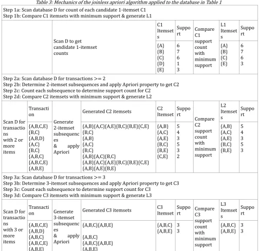
The Join-less Apriori Algorithm [9] modified the apriori algorithm to avoid the join stage of the classical algorithm. In the kth database scan of the join-less
apriori algorithm, all k-1 subsets of every transaction with length l (l ≥ k) are determined, and the apriori propertey applied to prune every candidate k-itemset with one or more infrequent (k-1)-itemsets.
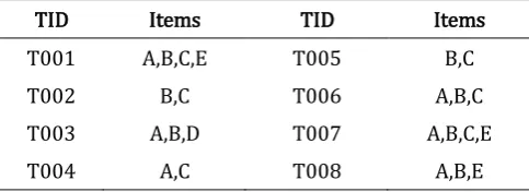
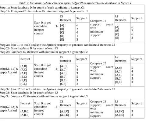
We next illustrate the working of both the classical and joinless apriori algorithms. Consider the transactions database D, Table 1, and the minimum support count to be 3. The steps required to generate frequent itemsets using the classical and joinless apriori algorithms are illustrated in Tables 2 and 3 respectively.
Table 1: Sample transactions database
TID Items TID Items
T001 A,B,C,E T005 B,C
T002 B,C T006 A,B,C
T003 A,B,D T007 A,B,C,E
Table 2: Mechanics of the classical apriori algorithm applied to the database in Figure 1
Step 1a: Scan database D for count of each candidate 1-itemset C1 Step 1b: Compare C1 itemsets with minimum support & generate L1
Scan D to get candidate 1-itemset
counts
C1
Itemsets Support Compare C1 support count with
minimum support
L1
Itemsets Support {A}
{B} {C} {D} {E}
6 7 6 1 3
{A} {B} {C} {E}
6 7 6 3 Step 2a: Join L1 to itself and use the Apriori property to generate candidate 2-itemsets C2
Step 2b: Scan database D for count of each C2
Step 2c: Compare C2 itemsets with minimum support & generate L2
Join(L1, L1) & apply Apriori
Itemset
Scan D to get candidate 2-itemset
counts
C2
itemsets Support
Compare C2 support count with
minimum support
L2
Itemsets Support {A,B}
{A,C} {A,E} {B,C} {B,E} {C,E}
{A,B} {A,C} {A,E} {B,C} {B,E} {C,E}
5 4 3 5 3 2
{A,B} {A,C} {A,E} {B,C} {B,E}
5 4 3 5 3 Step 3a: Join L2 to itself and use the Apriori property to generate candidate 2-itemsets C3
Step 3b: Scan database D for count of each C3
Step 3c: Compare C3 itemsets with minimum support & generate L3
Join(L2, L2) & apply Apriori
Itemset Scan D to get candidate 3-itemset
counts
C3
Itemsets Support
Compare C3 support count with
minimum support
L3
Itemsets Support {A,B,C}
{A,B,E}
{A,B,C} {A,B,E}
3 3
{A,B,C} {A,B,E}
3 3
3. DESIGN OF DATA STRUCTURES FOR THE VECTOR SPACE MODEL AND APRIORI ALGORITHMS
Before presenting the data structures that were used in our implementations, we give general principles that guided our choices. The first observation is that because the amount of data required is generally unknown until run time, the required memory to hold the data needs to be allocated dynamically; that leaves us with linked lists and BSTs. We next need to decide when to choose BSTs and when to choose linked lists. The choice was guided by an examination of the costs involved, as summarized below.
Unsorted linked list. Cost of inserting a node is low, as we just insert at the head of the list. However, search cost is high because of the sequential access to nodes, especially if the item searched for is not on the list.
Search cost may be unacceptably high if the list is very long.
Sorted linked list. Cost of inserting a node is higher than for an unsorted list, since we need to first traverse the list up to the suitable position before adding a new item. On the other hand, search cost is lower on average than for an unsorted list. Nevertheless, search cost may still be unacceptably high if the list is very long
Table 3: Mechanics of the joinless apriori algorithm applied to the database in Table 1
Step 1a: Scan database D for count of each candidate 1-itemset C1 Step 1b: Compare C1 itemsets with minimum support & generate L1
Scan D to get candidate 1-itemset counts C1 Itemset s Suppo
rt Compare C1 support count with minimum support L1 Itemset s Suppo rt {A} {B} {C} {D} {E} 6 7 6 1 3 {A} {B} {C} {E} 6 7 6 3
Step 2a: Scan database D for transactions >= 2
Step 2b: Determine 2-itemset subsequences and apply Apriori property to get C2 Step 2c: Count each subsequence to determine support count for C2
Step 2d: Compare C2 itemsets with minimum support & generate L2
Scan D for transactio ns with 2 or more items Transacti on Generate 2-itemset subsequenc es
& apply Apriori
Generated C2 itemsets C2 Itemset Suppo rt Compare C2 support count with minimum support L2 Itemset s Suppo rt {A,B,C,E} {B,C} {A,B,D} {A,C} {B,C} {A,B,C} {A,B,C,E} {A,B,E} {A,B}{A,C}{A,E}{B,C}{B,E}{C,E} {B,C} {A,B} {A,C} {B,C} {A,B}{A,C}{B,C} {A,B}{A,C}{A,E}{B,C}{B,E}{C,E} {A,B}{A,E}{B,E} {A,B} {A,C} {A,E} {B,C} {B,E} {C,E} 5 4 3 5 3 2 {A,B} {A,C} {A,E} {B,C} {B,E} 5 4 3 5 3
Step 3a: Scan database D for transactions >= 3
Step 3b: Determine 3-itemset subsequences and apply Apriori property to get C3 Step 3c: Count each subsequence to determine support count for C3
Step 3d: Compare C3 itemsets with minimum support & generate L3
Scan D for transactio ns with 3 or more items
Transacti
on Generate 3-itemset subsequenc es
& apply Apriori
Generated C3 itemsets C3 Itemset
Suppo
rt Compare C3 support count with minimum support L3 Itemset s Suppo rt {A,B,C,E} {A,B,D} {A,B,C} {A,B,C,E} {A,B,E} {A,B,C}{A,B,E} {A,B,C} {A,B,C}{A,B,E} {A,B,E} {A,B,C} {A,B,E} 3 3 {A,B,C} {A,B,E} 3 3
3.1. Creating the Vector-space Model
Key objectives in the creation of the VSM are first, the creation of an inverted file, which comprises a dictionary of index terms, and for each index term, a list of the documents (i.e., the postings list) that the term occurs in, and second, the creation of document vectors for each document in the collection. Corresponding term and document statistics are also collected as follows:
Term statistics: For each term, statistics on term frequency across the collection (TF), list of documents containing the term, and for each such document, the document term frequency (DTF), i.e., the number of terms in the document.
Document statistics: For each document containing a given term, statistics on the number of terms in the document, the list of terms that constitute the document, and for each such term, the frequency of the term in the document.
on computers with only a moderate amount of RAM. We summarize the steps involved in the processing in Figure 1.
3.2. Choice of Data Structures for the Vector-space Model
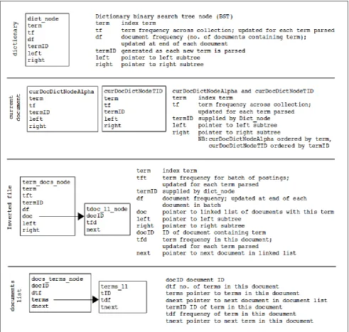
Dictionary. Obvious candidates for data structure to represent the dictionary are a linked list or a binary search tree (BST). But because of the need to search the data structure to update term statistics or to create a new node for each new term, a BST, ordered by the string representing each term, was used. Every node of the tree comprises the following data fields: term, term ID, term frequency (i.e., number of occurrences across the document collection), the document frequency (i.e., number of documents containing the term).
The inverted file. As with the dictionary, the inverted file needs to be searched during document parsing, and so a BST is used to hold its data. Every node of this tree comprises fields for the term, term ID, term frequency and document frequency. Additionally, there is a linked list to all the documents that the term belongs to. Each node in this linked list comprises fields for the document ID and the frequency of that term in the document. We note that a linked list is good enough for the document list because (1) the parsed document set is normally already arranged in order of document ID,
and any BST created to track documents containing the term would degenerate into a linked list; and (2) no search is required on this document list.
Documents list. Required document statistics are also collected as each document is parsed. A linked list is used to represent the various documents parsed. Again, because there is no need to search this list, and the documents are already arranged in document ID order, the choice of linked list is appropriate. Each node on this list comprises fields for the document ID and the number of terms in the document. Additionally, each node maintains a linked list of terms that are found in the document. This linked list tracks corresponding term IDs and their corresponding frequencies in the document. For ease of processing, terms are added to this list in term ID order.
Current document. As each document is parsed, its terms are read into two BSTs: curDocDictNodeAlpha
and curDocDictNodeTID. These BSTs have identical nodes with fields for the term, term ID, and term frequency across the document collection, updated for each term parsed. The only difference between these two BSTs is that the former is ordered by term name and the latter by term ID. As each term is parsed, the term frequency on these BSTs and the document list are updated.
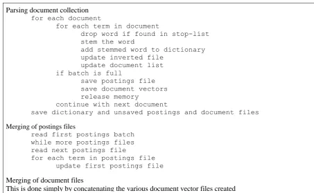
Figure 1: Vector-space Model – Generation of Postings and Document Files
Parsing document collection
for each document
for each term in document
drop word if found in stop-list stem the word
add stemmed word to dictionary update inverted file
update document list if batch is full
save postings file save document vectors release memory
continue with next document
save dictionary and unsaved postings and document files
Merging of postings files
read first postings batch while more postings files read next postings file
for each term in postings file update first postings file
Merging of document files
Figure 2: Data structures used in constructing the vector-space model
Then, at the end of each document parsed: curDocDictNodeAlpha is used to update the document frequencies of corresponding terms in both the dictionary BST and the inverted file, while curDocDictNodeTID is used to maintain the terms linked list in documents list. The advantage of using curDocDictNodeTID over curDocDictNodeAlpha in the second case is that the terms are accessed in term ID order, the same order we would like them in the document vector. The data structures used are summarized in Figure 2.
3.3. Frequent Itemsets Mining using the Apriori Algorithm
algorithm, it is important to be able to organize the itemsets as well as the terms constituting the itemsets to be joined in a manner that minimizes the number of computations to be done. Finally, the generation of subsets from itemsets must be efficient. This is because the apriori property which requires generation of subsets is applied so many times in the mining process.
3.4 Choice of Data Structures for Frequent Itemsets Mining using the Apriori Algorithm
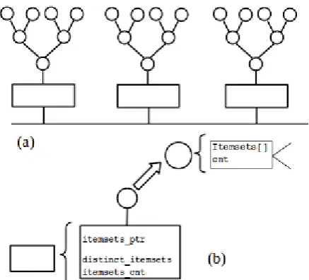
Figure 3 illustrates the data structure used to store itemsets. The data structure is a hash table, with each entry in the table comprising a node with a pointer to a BST. Use of a hash table reduces the search space for itemsets by limiting search for all itemsets that hash to the same value to the corresponding hash table entry.
Figure 3: Hash table to store candidate and frequent itemsets: (a) table skeleton; (b) node details.
The node at each hash table cell keeps track of the following statistics for the corresponding itemsets:
distinct_itemsets – the number of distinct itemsets, and
itemset_cnt – the cumulative total of all the itemsets. The pointer itemset_ptr links to a binary search tree that holds all itemsets that hash to the same value. Every node on the itemsets BST keeps track of the following data: a k-itemset stored in a dynamically allocated array that holds the itemset data, and cnt, the number of occurences of the k-itemset.
The join step at stage k of the classical apriori algorithm requires joining the frequent (k-1)-itemsets vector to itself. It helps the computation if the items in each itemset are arranged in lexicographic order. To achieve this need, (1) the itemsets in the transaction database are pre-arranged to be in lexicographic order, and (2) the itemsets to be joined are read from the BST
in-order, into a linked list, before the join operation.
This is important as it ensures that the items in each itemset on the list are in lexicographic order, a required condition for the joining of itemsets.
4. CONCLUSION
In this paper, we have reviewed some of the most commonly used data structures and highlighted performance issues related to their use. We have also reviewed two important problems: generation of the vector-space model for document representations, and mining of frequent itemsets using the apriori algorithm. Finally, we have illustrated our choices of data structures and algorithms used in our implementations of solutions to the two classes of problems mentioned. 5. REFERENCES
[1] R. Sedgewick, Algorithms in C, Parts 1-4: Fundamentals, Data Structures, Sorting, Searching, 3rd edition. Reading, Mass: Addison-Wesley Professional, 1997.
[2] R. Neapolitan and K. Naimipour, Foundations of Algorithms, 4th edition. Sudbury, Mass: Jones & Bartlett Learning, 2009.
[3] R. Agrawal, T. Imieliński, and A. Swami, “Mining Association Rules Between Sets of Items in Large Databases,” in Proceedings of the 1993 ACM SIGMOD International Conference on Management of Data, New York, NY, USA, 1993, pp. 207–216. [4] R. Agrawal and R. Srikant, “Fast Algorithms for
Mining Association Rules in Large Databases,” in
Proceedings of the 20th International Conference on Very Large Data Bases, San Francisco, CA, USA, 1994, pp. 487–499.
[5] H. Mannila, H. Toivonen, and A. I. Verkamo, “Efficient Algorithms for Discovering Association Rules,” in Proceedings of the 3rd International Conference on Knowledge Discovery and Data Mining, Seattle, WA, 1994, pp. 181–192.
[6] I. Han and M. Kamber, “Data mining concepts and techniques,” Morgan Kaufinann, 2006.
[7] I. H. Witten, E. Frank, and M. A. Hall, Data Mining: Practical Machine Learning Tools and Techniques, 3rd edition. Burlington, MA: Morgan Kaufmann, 2011.
[8] J. Dongre, G. L. Prajapati, and S. V. Tokekar, “The role of Apriori algorithm for finding the association rules in Data mining,” in 2014 International Conference on Issues and Challenges in Intelligent Computing Techniques (ICICT), 2014, pp. 657–660.
(PRIS-2004), 2005, pp. 234–243.
[10] T. W. Parsons, Introduction to Algorithms in Pascal, 1st edition. New York: Wiley, 1994.
[11] R. Baeza-Yates and B. Ribeiro-Neto, Modern Information Retrieval, 1st edition. New York : Harlow, England: Addison Wesley, 1999.
[12] R. R. Korfhage, Information Storage and Retrieval, 1st edition. New York: Wiley, 1997.
[13] D. A. Grosman and O. Frieder, Information Retrieval - Algorithms and Heuristics. Springer, 1998.
[14] M. Sanderson and W. B. Croft, “The History of Information Retrieval Research,” Proc. IEEE, vol. 100, no. Special Centennial Issue, pp. 1444–1451, May 2012.
[15] S. Rueger and G. Marchionini, Multimedia Information Retrieval, 1st edition. San Rafael, Calif.: Morgan and Claypool Publishers, 2010. [16] W. S. Cooper, “Getting Beyond Boole,” Inf Process
Manage, vol. 24, no. 3, pp. 243–248, May 1988. [17] C. D. Manning, P. Raghavan, and H. Schütze,
Introduction to Information Retrieval. Cambridge University Press, 2008.
[18] G. Salton, A. Wong, and C. S. Yang, “A Vector Space Model for Automatic Indexing,” Commun ACM, vol. 18, no. 11, pp. 613–620, Nov. 1975.
[19] G. Salton, Automatic Text Processing: The Transformation, Analysis, and Retrieval of Information by Computer. Boston, MA, USA: Addison-Wesley Longman Publishing Co., Inc., 1989.
[20] G. Salton and M. J. McGill, Introduction to Modern Information Retrieval. New York, NY, USA: McGraw-Hill, Inc., 1986.
[21] T. Mikolov, K. Chen, G. Corrado, and J. Dean, “Efficient estimation of word representations in vector space,” ArXiv Prepr. ArXiv13013781, 2013. [22] T. Mikolov, I. Sutskever, K. Chen, G. S. Corrado, and
J. Dean, “Distributed Representations of Words and Phrases and their Compositionality,” in
Advances in Neural Information Processing Systems 26, C. J. C. Burges, L. Bottou, M. Welling, Z. Ghahramani, and K. Q. Weinberger, Eds. Curran Associates, Inc., 2013, pp. 3111–3119.
[23] P. D. Turney and P. Pantel, “From Frequency to Meaning: Vector Space Models of Semantics,”
ArXiv10031141 Cs, Mar. 2010.
[24] S. Sharma and V. Gupta, “Recent developments in text clustering techniques,” Recent Dev. Text Clust. Tech., vol. 37, no. 6, 2012.
[25] P. P. Senellart and V. D. Blondel, “Automatic Discovery of Similar Words,” in Survey of Text Mining, M. W. Berry, Ed. New York, NY: Springer New York, 2004, pp. 25–43.
[26] M. Kobayashi and M. Aono, “Vector Space Models for Search and Cluster Mining,” in Survey of Text Mining II, M. W. Berry and M. Castellanos, Eds. London: Springer London, 2008, pp. 109–127. [27] Q. Yang and X. Wu, “10 Challenging Problems in
Data Mining Research,” Int. J. Inf. Technol. Amp Decis. Mak., Nov. 2011.
[28] R. Kosala and H. Blockeel, “Web Mining Research: A Survey,” SIGKDD Explor Newsl, vol. 2, no. 1, pp. 1–15, Jun. 2000.
[29] M. Mohania and A. M. Tjoa, Eds., DataWarehousing and Knowledge Discovery, vol. 1676. Berlin, Heidelberg: Springer Berlin Heidelberg, 1999. [30] R. S. J. d Baker and K. Yacef, “The State of
Educational Data Mining in 2009: A Review and Future Visions,” JEDM - J. Educ. Data Min., vol. 1, no. 1, pp. 3–17, Oct. 2009.
[31] J. Hipp, U. Güntzer, and G. Nakhaeizadeh, “Algorithms for Association Rule Mining — a General Survey and Comparison,” SIGKDD Explor Newsl, vol. 2, no. 1, pp. 58–64, Jun. 2000.
[32] C. Zhang and S. Zhang, Association Rule Mining: Models and Algorithms. Berlin, Heidelberg: Springer-Verlag, 2002.