Vol.9 (2019) No. 6
ISSN: 2088-5334
Monte Carlo Tree Search in Finding Feasible Solutions for Course
Timetabling Problem
Say Leng Goh
#, Graham Kendall
*, Nasser R. Sabar
+ #Decision Sciences Lab, ISRG, Faculty of Computing and Informatics, Universiti Malaysia Sabah Labuan International Campus, Labuan, 87000, Malaysia.
E-mail: [email protected]
*
School of Computer Science, The University of Nottingham Malaysia Campus, Semenyih, Malaysia. E-mail: [email protected]
+
Department of Computer Science and Information Technology, La Trobe University, Melbourne, Australia. E-mail: [email protected]
Abstract— We are addressing the course timetabling problem in this work. In a university, students can select their favorite courses each semester. Thus, the general requirement is to allow them to attend lectures without clashing with other lectures. A feasible solution is a solution where this and other conditions are satisfied. Constructing reasonable solutions for course timetabling problem is a hard task. Most of the existing methods failed to generate reasonable solutions for all cases. This is since the problem is heavily constrained and an effective method is required to explore and exploit the search space. We utilize Monte Carlo Tree Search (MCTS) in finding feasible solutions for the first time. In MCTS, we build a tree incrementally in an asymmetric manner by sampling the decision space. It is traversed in the best-first manner. We propose several enhancements to MCTS like simulation and tree pruning based on a heuristic. The performance of MCTS is compared with the methods based on graph coloring heuristics and Tabu search. We test the solution methodologies on the three most studied publicly available datasets. Overall, MCTS performs better than the method based on graph coloring heuristic; however, it is inferior compared to the Tabu based method. Experimental results are discussed.
Keywords— combinatorial optimization; timetabling; monte carlo tree search; graph coloring heuristics; tabu search.
I. INTRODUCTION
Course timetabling problem (CTP) involves allocating courses to time slots and rooms to produce a satisfactory timetable satisfying several constraints. CTP is a variant of the combinatorial optimization problem (COP). It is a widely studied NP-complete problem due to its practical importance to universities. A feasible course timetable prevents clashes of courses allowing students to attend all the lectures for courses registered. As a result, lecturers are not required to conduct replacement classes for the clashing courses. A feasible timetable ensures that lecture rooms fulfill the requirements of courses by having enough seats and teaching equipment such as overhead projector, audio/video, Internet connection etc. By having a feasible timetable, it is possible to conduct courses (possibly related) in a specific sequence. For instance, some courses may require that lectures be conducted before tutorials or vice-versa. Finally, a feasible
course timetable allows busy lecturers to perform courses at certain preferred times.
MCTS is considered as a comparatively new search methodology. It has caught the attention of the Artificial Intelligence (AI) community because of its success in the games area. The impact of MCTS in the territory of the game has inspired us to figure out the performance of MCTS in CTP which are dominated by local search methods. We apply MCTS in finding feasible solutions (solutions that fulfill all the hard constraints) for the first time. We propose several enhancements to MCTS, such as simulation and tree pruning based on a heuristic. The performance of MCTS is compared with that of the classical graph coloring approach as well as Tabu Search.
A. Problem Description
namely, student can only attend one course at one time, a room must fulfill the features required by a course, a room must provide enough seats for a course, and only one course is allowed in every time slot and room. ITC07 has two extra hard constraints consist of a course that must be assigned to one of the preset time slots and a course may be required to appear in a certain sequence.
B. Related Work
MCTS based programs are now comparable with the best human players [1], [2], [3]. MCTS is well known in games AI but it is seldom used for COP. Examples of the application of MCTS in COP are job shop scheduling [4], one player puzzle [5], reentrant scheduling problem [6] and production management problems [7]. To our knowledge, MCTS has never been utilized on CTP.
Various approaches have been developed in finding feasible solutions for CTP. One common approach is utilizing graph coloring heuristics. A hybrid of graph coloring heuristics was employed to construct an early solution by Sabar et al. where events were randomly assigned to time slots and rooms after sorting them by heuristics such as largest degree, largest enrolment and saturation degree [8]. Interested readers may refer to [9] and [10].
Another common approach is based on Tabu search. To find a feasible solution, Cambazard et al. performed a local search on randomly generated solutions [11]. In order to avoid an event from being repeatedly allocated the identical time slots, a Tabu list is maintained for certain number of iterations. They used neighborhood structures such as transferring a course to a vacant place, exchanging two courses, exchanging two-time slots, matching (courses are unassigned and reassigned within a time slot), transferring a course using matching and Hungarian move. Other examples of this approach can be found in [12] and [13]. Some authors are using methods based on the combination of graph coloring heuristics and Tabu search in finding feasible solutions. 100% feasibility is attained for all the cases of ITC07 by Lewis and Thompson using constructive heuristics and then PARTIALCOL algorithm [14]. Unassigned events were handled using a Tabu mechanism [15]. Refer to [16] and [17] for other similar methods.
II. MATERIALS AND METHOD A. MCTS
In MCTS, every state is constituted by a node in the tree and a directed link constitutes every action (leading to the state). Every node contains a value and a visit count. MCTS comprises four key steps specifically selection, expansion, simulation and back-propagation. These steps are repeated within available computation resources. Inside the selection step, the tree is covered from the root until a non-terminal node (with unvisited action) arrives. Inside the expansion step, a new child node is appended for the unvisited action. Inside the simulation step, a playout is carried out from the child node to generate an outcome. Inside the backpropagation step, the covered nodes (plus the child node) are updated with values from the outcome. Finally, the best child (child node having the greatest average value or visit
count) of the root node is the selected move. The process is depicted in Fig. 1, from [18].
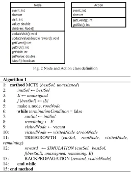
Fig. 1 MCTS
In our MCTS implementation, we assign events into time slots and use maximal matching for room assignment. The node and action classes are defined as shown in Fig. 2. Algorithm 1 shows the MCTS method. We set the initial solution initSol to best solution bestSol, list of events E to unassigned events uassigned and best cost f(bestSol) to the number of events in E. We make a node as the root node
rootNode. The iteration stops when the
terminationCondition is true (when either we found a
feasible solution or the elapsed time passes execution time t). At the start of every iteration, we set the current solution
curSol to initSol, the list of remaining events remaining to
events in E and the list of visited nodes visitedNode to vacant. We append the root node to visitedNode. Nodes visited during tree traversal are kept in the visitedNode.
Fig. 2 Node and Action class definition
Algorithm 1
1: method MCTS (bestSol, unassigned) 2: initSol ← bestSol
3: E ← unassigned
4: f (bestSol) ← |E|
5: make a node, rootNode
6: while terminationCondition = false 7: curSol ← initSol
8: remaining ← E
9: visitedNode ← vacant
10: visitedNode ← visitedNode ∪ rootNode
11: TREEGROWTH (curSol, rootNode, visitedNode,
remaining)
12: reward ← SIMULATION (curSol, bestSol, f(bestSol), unassigned, remaining, E)
13: BACKPROPAGATION (reward, visitedNode) 14: end while
TREEGROWTH method is given in Algorithm 2. We set the currentNode to rootNode. While currentNode is not a leaf node, we select one of the children of currentNode as the current node by using the SELECTION method in Algorithm 7. We then append the current node to
visitedNode. The event of currentNode is assigned to curSol
according to the time slot of currentNode. We then remove that event from remaining. We try to expand the tree from the leaf node if the currentNode is leaf node. All the possible actions are selected and stored in the list of actions A by the GETACTIONS method (Algorithm 8). If A is not vacant, we append all actions in A as the children of currentNode using the EXPANSION method (Algorithm 11). We randomly choose one of the children as the child node childNode and append it to visitedNode. The event of childNode is assigned to curSol according to the time slot of childNode. We then remove that event from remaining.
Algorithm 2
1: method TREEGROWTH (curSol, rootNode, visitedNode,
remaining)
2: currentNode ← rootNode
3: while currentNode is not leaf
4: currentNode ← SELECTION (currentNode)
5: visitedNode ← visitedNode ∪ currentNode
6: curSol ← curSol ∪ currentNode.event
7: remaining ← remaining − currentNode.event
8: end while
9: A ←GETACTIONS (remaining, curSol) 10: if A is not vacant
11: EXPANSION (currentNode, A)
12: childNode ← select one of currentNode.children
randomly
13: visitedNode ← visitedNode ∪ childNode
14: curSol ← curSol ∪ childNode.event
15: remaining ← remaining − childNode.event
16: end if 17: end method
SIMULATION method is presented in Algorithm 3. We assign events to time slots in curSol. An event in remaining is returned according to heuristics by SELECTEVENT. SELECTTIMESLOT returns a time slot that is suitable for
event. Dynamic Search Rearrangement (DSR) is used for
event and time slot selection as it is the most effective heuristic based on experience. unplaced is a list of unplaced events that keeps events without any compatible time slot. We calculate f(curSol) as the number of events in unplaced.
bestSol, f(bestSol) and unassigned are updated if f(curSol) is
superior than f(bestSol). As reward is specified as the ratio of assigned events to the number of events, reward in the range of 0 to 1 is returned.
Algorithm 3
1: method SIMULATION (curSol, bestSol, f(bestSol), unassigned, remaining, E)
2: unplaced ← vacant
3: size ← |remaining|
4: for i = 1 to size
5: event ← SELECTEVENT (remaining, curSol)
6: timeSlot ← SELECTTIMESLOT (event, remaining, curSol)
7: if timeSlot is not null
8: curSol ← curSol ∪ event //assign event to timeSlot
9: else
10: unplaced ← unplaced ∪ event
11: end if
12: remaining ← remaining − event
13: end for
14: f (curSol) ← |unplaced|
15: if f (curSol) < f (bestSol) 16: bestSol ← curSol
17: f (bestSol) ← f (curSol)
18: unassigned ← unplaced
19: end if
20: return (|E|−|unplaced|) / |E| 21: end method
BACKPROPAGATION method is shown in Algorithm 4. We update the visit and value attribute of every node in
visitedNode. We increment the visit count and update the
value as a cumulative mean of reward.
Algorithm 4
1: method BACKPROPAGATION (reward, visitedNode) 2: for all node in visitedNode
3: node.updateVisit()
4: node.updateValue(reward)
5: end for 6: end method
We describe the SELECTION, GETACTIONS and EXPANSION methods stated earlier in detail below. In SELECTION method (Algorithm 5), we return a child with the highest UCB value among the children of currentNode. We balance the search exploration and exploitation by adjusting the constant B. More priority is given to the less frequently visited nodes when B is set higher. We set B as 0.0001.
Algorithm 5
1: method SELECTION (currentNode)
2: return arg maxi∈children of currentNode valuei +
B
3: end method
GETACTIONS method is given Algorithm 6. To avoid the tree from getting too wide, we apply several heuristics used in graph coloring to filtrate the actions. Effectively, we prune the tree based on heuristics. Bear in mind that an action comprises of an event and a time slot. Events in
remaining are returned based on heuristics by GETEVENTS.
GETTIMESLOTS returns time slots that are suitable for e.
Algorithm 6
1: method GETACTIONS (remaining, curSol) 2: A ← vacant
3: E ← GETEVENTS (remaining, curSol)
4: for all e in E
5: TS ← GETTIMESLOTS (e, remaining, curSol)
6: for all ts in TS
7: A ← A ∪ action (e, ts)
EXPANSION method is shown in Algorithm 7. We append all actions in A as children of currentNode. Unlike the general implementation of MCTS (where a child node is appended whenever an unvisited action is encountered), we append multiple nodes at one time. Our intention is to save computation cost with the sacrifice of some memory.
Algorithm 7
1: method EXPANSION (currentNode, A)
2: append all actions in A as children of currentNode 3: end method
B. Benchmark: Graph Colouring Heuristic (GCH)
In the graph coloring problem, GCH is considered a classical approach. The heuristics derived from graph coloring problem are often utilized in CTP. Usually, difficult events are assigned first with the hope that easier events will be assigned later as the environment getting more restricted. Algorithm 8 presents the GCH method. At every iteration, an event is selected and assigned to a selected time slot. It is a one-pass method. In our experiments, Dynamic Search Rearrangement (DSR) [19] is utilized. DSR is a heuristic often used in constraint satisfaction problem. It is dynamic as the next selected event is determined at every iteration. In DSR, we select an event randomly from the set E={events with the least number of suitable time slots}. Next, we select a timeSlot randomly from the set P={time slots suitable for
event and fit the least number of left events}.
Algorithm 8
1: method GCH (bestSol, unasssigned) 2: remaining ← unassigned
3: unplaced ← vacant
4: size ← |remaining|
5: for i = 1 to size
6: event ← SELECTEVENT (remaining)
7: timeSlot ← SELECTTIMESLOT (event)
8: if timeSlot is not null
9: bestSol ← bestSol ∪ event //assign event to timeSlot
10: else
11: unplaced ← unplaced ∪ event 12: end if
13: remaining = remaining − event
14: end for
15: unassigned ← unplaced
16: end method
C. Benchmark: Tabu Search (TS)
PARTIALCOL [14] was originally utilized in addressing graph coloring problems. [16], [20] and [15] adapted the algorithm in solving CTP. The TS method we tested here is based on PARTIALCOL. A neighbor move is a move of one event from unplaced to a time slot in curSol. At every iteration, we evaluate all the neighborhood moves by taking into consideration all suitable non-Tabu time slots for entire events in unplaced. All events conflicting with e (precedence or clash constraint) are temporarily shifted from curSol to
unplaced in order to move an event e into a time slot feasibly.
Maximal matching is used for room assignment sparingly as it is computationally expensive. A room is selected randomly among the suitable rooms and the relevant event is shifted from curSol to unplaced in case matching could not find a room for the specific event. We assess solutions
(curSol, canSol, bestSol) utilizing the cost function f based on the number of unplaced events as given in Equation 1:
(1)
We record the neighbor move with the lowest candidate cost f(canSol) as bestEvent and bestSlot. We move the events conflicting with bestEvent from curSol to unplaced. We applied the best neighbor move by moving the bestEvent from unplaced to the bestSlot of curSlot. If f(curSlot) is superior than f(bestSol), bestSol, f(bestSol) and unassigned are updated. We prevent the events conflicting with
bestEvent from returning to their original time slots for some
iterations by utilizing the Tabu tenure in Equation 2:
RANDOM [10) +|unplaced| (2)
where |unplaced| is the number of unplaced events. We use the value 10 for the random element as the same value was used in [14], [15] and [20] and more importantly, it works well for all the datasets that we are working on. The value of Tabu tenure determines the level of search exploration. Most of the available moves are not reachable thus restricting the search when the value of Tabu tenure is set too high. Meanwhile, cycling tends to occur which may stall the search when the value is set too low. The iteration stops when a feasible solution is found (unplaced is vacant) or the elapsed time passes execution time t.
III. RESULTS AND DISCUSSION
We conducted the experiments on Intel Xeon (3.1GHz) with 4Gb RAM machines. We coded the algorithms utilizing Java language. The computation time limit (which is set by executing a benchmark program) for every execution is
T=190 seconds.
A. Random Simulation vs. Heuristic Based Simulation
TABLEI
HEURISTIC BASED VS RANDOM SIMULATION ON SOCHA CASES.SHOWN IS (MEANUNASSIGNED,BEST UNASSIGNED) FOR N=31EXECUTIONS.
Case Simulation
DSR Random
Small01 (0.00, 0) (0.00, 0)
Small02 (0.00, 0) (0.00, 0)
Small03 (0.00, 0) (0.00, 0)
Small04 (0.00, 0) (0.00, 0)
Small05 (0.00, 0) (0.00, 0)
Medium01 (0.00, 0) (4.42, 3)
Medium02 (0.00, 0) (6.06, 5)
Medium03 (0.00, 0) (10.71, 8)
Medium04 (0.00, 0) (3.71, 2)
Medium05 (0.00, 0) (13.10, 10)
Large (0.00, 0) (35.94, 34)
Avg. (0.00, -) (6.72, -)
TABLEII
HEURISTIC BASED VS RANDOM SIMULATION ON ITC02CASES.SHOWN IS (MEANUNASSIGNED,BEST UNASSIGNED) FOR N=31EXECUTIONS.
Case Simulation
DSR Random
01 (0.00, 0) (14.52, 12)
02 (0.00, 0) (10.74, 9)
03 (0.00, 0) (11.48, 10)
04 (0.00, 0) (20.16, 18)
05 (0.00, 0) -
06 (0.00, 0) -
07 (0.00, 0) (10.68, 9)
08 (0.00, 0) (12.71, 10)
09 (0.00, 0) (10.35, 6)
10 (0.00, 0) (17.13, 14)
11 (0.00, 0) (15.29, 13)
12 (0.00, 0) (19.26, 17)
13 (0.00, 0) (15.26, 13)
14 (0.00, 0) (16.06, 15)
15 (0.00, 0) (14.52, 13)
16 (0.00, 0) (5.68, 2)
17 (0.00, 0) -
18 (0.00, 0) (10.00, 7)
19 (0.00, 0) (13.90, 12)
20 (0.00, 0) (6.35, 5)
Avg. (0.00, -) (13.18, -)
TABLEIII
HEURISTIC BASED VS RANDOM SIMULATION ON ITC07CASES.SHOWN IS (MEANUNASSIGNED,BEST UNASSIGNED) FOR N=31EXECUTIONS.
Case Simulation
DSR Random
01 (15.90, 14) (73.39, 67)
02 (25.19, 20) -
03 (0.00, 0) -
04 - -
05 - -
06 (5.55, 2) -
07 - -
08 (0.00, 0) -
09 (24.77, 22) (78.97, 76)
10 (32.58, 29) (89.58, 86)
11 (0.00, 0) -
12 - -
13 (9.39, 7) -
14 - -
15 (0.00, 0) -
16 (0.00, 0) -
17 (0.00, 0) -
18 - -
19 - -
20 (0.00, 0) (36.58, 34)
21 (3.35, 2) (67.23, 65)
22 (54.58, 52) (131.39, 127)
23 - -
24 - -
Avg. (11.42, -) (79.52, -)
B. Heuristic Based Tree Pruning
We attempt to prune the tree in MCTS to address the memory issue faced earlier. We expand the tree by using a certain number of actions (an action involves assigning an event to a time slot) instead of all actions at one time (as in the previous section). Several heuristic-based pruning mechanisms is compared in this section. The idea is inspired by the work in [23], [24], [25] where the authors utilized domain knowledge for pruning. We present the descriptions of the heuristics based on Algorithm 8 in Table IV. Note that simulation based on DSR is used here due to its effectiveness, as shown in the previous section.
TABLEIV TREE PRUNING HEURISTICS.
Heuristics Description
DSR
All events having the least number of suitable time slots, E={e1,e2,...em} is returned by GETEVENTS method.
All-time slots suitable for em and fit the least number of
remaining events, S={s1,s2,...sn} are returned by
GETTIMESLOTS method.
LD-All
All events having the most number of clashes with other events, E={e1,e2,...em} is returned by GETEVENTS method.
All time slots suitable for em, S={s1,s2,...sn} are returned by
GETTIMESLOTS method.
MV-All
All events having the least number of suitable time slots, E={e1,e2,...em} is returned by GETEVENTS method.
All time slots suitable for em, S={s1,s2,...sn} are returned by
GETTIMESLOTS method.
SD-All
All events having the most number of clashes with other events, E2={e1,e2,...em} where E2 ⊂ E1 and E1={events with
the least number of suitable time slots} is returned by GETEVENTS method.
All time slots suitable for em, S={s1,s2,...sn} are returned by
GETTIMESLOTS method.
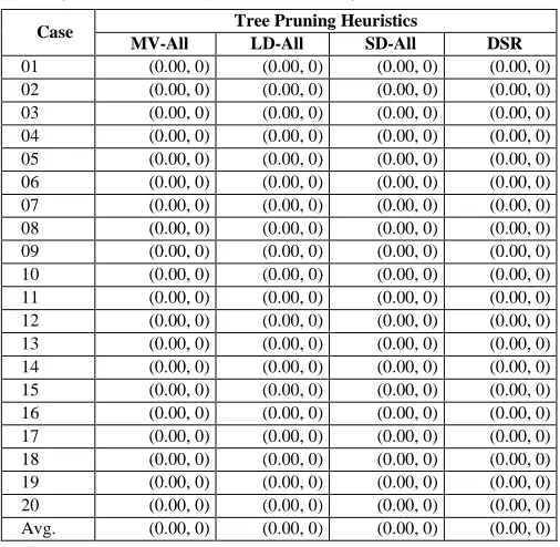
As shown in Table V and VI, 100% feasibility is attained for Socha and ITC02 cases regardless of heuristics applied for tree pruning. The same result is achieved even without pruning showing that these datasets are not challenging.
TABLEV
COMPARING TREE PRUNING HEURISTICS ON SOCHA CASES.SHOWN IS (MEAN UNASSIGNED,BEST UNASSIGNED) FOR N=31EXECUTIONS.
Case
Tree Pruning Heuristics
MV-All LD-All SD-All DSR
Large (0.00, 0) (0.00, 0) (0.00, 0) (0.00, 0) Avg. (0.00, 0) (0.00, 0) (0.00, 0) (0.00, 0)
TABLEVI
COMPARING TREE PRUNING HEURISTICS ON ITC02CASES.SHOWN IS (MEAN UNASSIGNED,BEST UNASSIGNED) FOR N=31EXECUTIONS.
Case Tree Pruning Heuristics
MV-All LD-All SD-All DSR
01 (0.00, 0) (0.00, 0) (0.00, 0) (0.00, 0) 02 (0.00, 0) (0.00, 0) (0.00, 0) (0.00, 0) 03 (0.00, 0) (0.00, 0) (0.00, 0) (0.00, 0) 04 (0.00, 0) (0.00, 0) (0.00, 0) (0.00, 0) 05 (0.00, 0) (0.00, 0) (0.00, 0) (0.00, 0) 06 (0.00, 0) (0.00, 0) (0.00, 0) (0.00, 0) 07 (0.00, 0) (0.00, 0) (0.00, 0) (0.00, 0) 08 (0.00, 0) (0.00, 0) (0.00, 0) (0.00, 0) 09 (0.00, 0) (0.00, 0) (0.00, 0) (0.00, 0) 10 (0.00, 0) (0.00, 0) (0.00, 0) (0.00, 0) 11 (0.00, 0) (0.00, 0) (0.00, 0) (0.00, 0) 12 (0.00, 0) (0.00, 0) (0.00, 0) (0.00, 0) 13 (0.00, 0) (0.00, 0) (0.00, 0) (0.00, 0) 14 (0.00, 0) (0.00, 0) (0.00, 0) (0.00, 0) 15 (0.00, 0) (0.00, 0) (0.00, 0) (0.00, 0) 16 (0.00, 0) (0.00, 0) (0.00, 0) (0.00, 0) 17 (0.00, 0) (0.00, 0) (0.00, 0) (0.00, 0) 18 (0.00, 0) (0.00, 0) (0.00, 0) (0.00, 0) 19 (0.00, 0) (0.00, 0) (0.00, 0) (0.00, 0) 20 (0.00, 0) (0.00, 0) (0.00, 0) (0.00, 0) Avg. (0.00, 0) (0.00, 0) (0.00, 0) (0.00, 0)
Memory issues are no longer faced when tree pruning is used in ITC07 cases. The maximum heap memory commitment during 31 executions for every problematic case in the previous section is presented in Table VII. Now, the maximum heap memory commitment is way below 1.5Gb (the allotted size). Note that we measured the heap memory sizes utilizing a tool supplied by Java Development Kit (JDK) called as Java Monitoring and Management Console.
TABLEVII
THE MAXIMUM MEMORY (MB)COMMITTED DURING 31EXECUTIONS FOR SELECTED ITC07CASES.
Case Maximum Heap Memory Commitment (Gb)
04 0.0272
05 0.1306
07 0.0241
12 0.0564
14 0.1471
18 0.0278
19 0.1587
23 0.1781
24 0.1343
Among the pruning heuristic tested, MV-All is the most promising one as feasible solutions were found for all cases exclude cases 1, 2, 9, 10 and 22 as evident in Table VIII. Excitingly, these results are compatible with those of a constraint programming approach [11] which also could not construct a feasible solutions for cases 1, 2, 9 and 10. The author did not consider case 22 in his experiment which is possibly hidden by the competition organizer at that point in time. From observation, we get better results when pruning is applied using any heuristic. With pruning, the tree size is considerably reduced. In effect, pruning eliminates poor
choices and guides the search to concentrate more time on finer options.
TABLEVIII
COMPARING TREE PRUNING HEURISTICS ON ITC07CASES.SHOWN IS (MEAN UNASSIGNED,BEST UNASSIGNED) FOR N=31EXECUTIONS.
Case Tree Pruning Heuristics
MV-All LD-All SD-All DSR
01 (6.39, 3) (7.13, 3) (6.87, 3) (6.94, 3) 02 (11.19, 6) (16.77, 11) (12.13, 9) (12.77, 7) 03 (0.00, 0) (0.00, 0) (0.00, 0) (0.00, 0) 04 (0.00, 0) (0.00, 0) (0.00, 0) (0.00, 0) 05 (0.03, 0) (0.23, 0) (0.16, 0) (1.84, 0) 06 (0.29, 0) (0.61, 0) (0.42, 0) (0.90, 0) 07 (0.00, 0) (0.00, 0) (0.03, 0) (0.13, 0) 08 (0.00, 0) (0.00, 0) (0.00, 0) (0.00, 0) 09 (16.97, 14) (17.61, 13) (15.16. 9) (14.39, 10) 10 (19.71, 15) (24.48, 17) (21.77, 16) (18.74, 14) 11 (0.00, 0) (0.00, 0) (0.00, 0) (0.00, 0) 12 (0.00, 0) (0.00, 0) (0.06, 0) (1.35, 0) 13 (1.13, 0) (2.29, 1) (1.26, 0) (2.58, 0) 14 (0.84, 0) (1.55, 0) (2.19, 0) (3.29, 1) 15 (0.00, 0) (0.06, 0) (0.00, 0) (0.10, 0) 16 (0.00, 0) (0.00, 0) (0.00, 0) (0.00, 0) 17 (0.00, 0) (0.00, 0) (0.00, 0) (0.00, 0) 18 (0.00, 0) (0.00, 0) (0.00, 0) (0.68, 0) 19 (2.77, 0) (3.16, 1) (8.26, 4) (10.61, 6) 20 (0.00, 0) (0.00, 0) (0.00, 0) (0.00, 0) 21 (1.10, 0) (1.03, 0) (0.39, 0) (0.74, 0) 22 (44.68, 41) (49.06, 46) (40.45, 31) (34.87, 28) 23 (6.16, 0) (13.97, 7) (9.23, 2) (8.77, 2) 24 (0.06, 0) (0.35, 0) (1.61, 0) (4.42, 1) Avg. (4.64, -) (5.76, -) (5.00, -) (5.13, -)
C. Comparing MCTS with GCH and TS
The attainment of MCTS, GCH, and TS in finding feasible solutions is compared in this section. The GCH considered here is based on the DSR heuristic. While for the MCTS, MV-All and DSR heuristics are utilized for the tree pruning and simulation phase respectively. As shown in Table IX, all three methods found feasible solutions for all Socha cases. Both MCTS and TS attained 100% feasibility.
TABLEIX
COMPARING MCTS,GCH, AND TS ON SOCHA CASES.SHOWN IS (FEASIBILITY %,MEAN UNASSIGNED,BEST UNASSIGNED) FOR N=31
EXECUTIONS.
Case MCTS GCH TS
Small01 (100, 0.00, 0) (100, 0.00, 0) (100, 0.00, 0) Small02 (100, 0.00, 0) (100, 0.00, 0) (100, 0.00, 0) Small03 (100, 0.00, 0) (100, 0.00, 0) (100, 0.00, 0) Small04 (100, 0.00, 0) (100, 0.00, 0) (100, 0.00, 0) Small05 (100, 0.00, 0) (100, 0.00, 0) (100, 0.00, 0) Medium01 (100, 0.00, 0) (6, 5.00, 0) (100, 0.00, 0) Medium02 (100, 0.00, 0) (29, 2.55, 0) (100, 0.00, 0) Medium03 (100, 0.00, 0) (74, 0.48, 0) (100, 0.00, 0) Medium04 (100, 0.00, 0) (10, 3.52, 0) (100, 0.00, 0) Medium05 (100, 0.00, 0) (71, 0.68, 0) (100, 0.00, 0) Large (100, 0.00, 0) (3, 6.48, 0) (100, 0.00, 0)
TABLEX
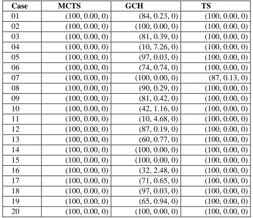
COMPARING MCTS,GCH, AND TS ON ITC02CASES.SHOWN IS (FEASIBILITY %,MEAN UNASSIGNED,BEST UNASSIGNED,) FOR N=31
EXECUTIONS.
Case MCTS GCH TS
01 (100, 0.00, 0) (84, 0.23, 0) (100, 0.00, 0) 02 (100, 0.00, 0) (100, 0.00, 0) (100, 0.00, 0) 03 (100, 0.00, 0) (81, 0.39, 0) (100, 0.00, 0) 04 (100, 0.00, 0) (10, 7.26, 0) (100, 0.00, 0) 05 (100, 0.00, 0) (97, 0.03, 0) (100, 0.00, 0) 06 (100, 0.00, 0) (74, 0.74, 0) (100, 0.00, 0) 07 (100, 0.00, 0) (100, 0.00, 0) (87, 0.13, 0) 08 (100, 0.00, 0) (90, 0.29, 0) (100, 0.00, 0) 09 (100, 0.00, 0) (81, 0.42, 0) (100, 0.00, 0) 10 (100, 0.00, 0) (42, 1.16, 0) (100, 0.00, 0) 11 (100, 0.00, 0) (10, 4.68, 0) (100, 0.00, 0) 12 (100, 0.00, 0) (87, 0.19, 0) (100, 0.00, 0) 13 (100, 0.00, 0) (60, 0.77, 0) (100, 0.00, 0) 14 (100, 0.00, 0) (100, 0.00, 0) (100, 0.00, 0) 15 (100, 0.00, 0) (100, 0.00, 0) (100, 0.00, 0) 16 (100, 0.00, 0) (32, 2.48, 0) (100, 0.00, 0) 17 (100, 0.00, 0) (71, 0.65, 0) (100, 0.00, 0) 18 (100, 0.00, 0) (97, 0.03, 0) (100, 0.00, 0) 19 (100, 0.00, 0) (65, 0.94, 0) (100, 0.00, 0) 20 (100, 0.00, 0) (100, 0.00, 0) (100, 0.00, 0)
Table XI presents the result comparison of the three methods applied to ITC07 cases. TS is the only methodology that can find feasible solutions for the entire cases. GCH obtained feasible solutions for 5 (cases 3, 8, 16, 17 and 20) out of the 24 cases. Meantime, MCTS obtained feasible solutions for all the cases exclude cases 1, 2, 9, 10 and 22. In truth, none of the methods could accomplish 100% feasibility for all the cases. TS performed competently with 100% feasibility for all the cases excluding cases 11, 19 and 23.
TABLEXI
COMPARING MCTS,GCH, AND TS ON ITC07CASES.SHOWN IS (FEASIBILITY %,MEAN UNASSIGNED,BEST UNASSIGNED) FOR N=31
EXECUTIONS.
Case MCTS GCH TS
01 (0, 6.39, 3) (0, 34.29, 26) (100, 0.00, 0) 02 (0, 11.19, 6) (0, 45.03, 36) (100, 0.00, 0) 03 (100, 0.00, 0) (10, 4.35, 0) (100, 0.00, 0) 04 (100, 0.00, 0) (0, 9.94, 4) (100, 0.00, 0) 05 (97, 0.03, 0) (0, 20.42, 13) (100, 0.00, 0) 06 (72, 0.29, 0) (0, 20.26, 11) (100, 0.00, 0) 07 (100, 0.00, 0) (0, 11.87, 6) (100, 0.00, 0) 08 (100, 0.00, 0) (3, 4.97, 0) (100, 0.00, 0) 09 (0, 16.97, 14) (0, 43.26, 32) (100, 0.00, 0) 10 (0, 19.71, 15) (0, 53.29, 43) (100, 0.00, 0) 11 (100, 0.00, 0) (0, 7.10, 1) (87, 0.26, 0) 12 (100, 0, 0.00) (0, 14.26, 4) (100, 0.00, 0) 13 (23, 1.13, 0) (0, 25.26, 17) (100, 0.00, 0) 14 (42, 0.84, 0) (0, 24.81, 16) (100, 0.00, 0) 15 (100, 0.00, 0) (0, 9.97, 5) (100, 0.00, 0) 16 (100, 0.00, 0) (10, 2.39, 0) (100, 0.00, 0) 17 (100, 0.00, 0) (42, 1.26, 0) (100, 0.00, 0) 18 (100, 0.00, 0) (0, 17.61, 10) (100, 0.00, 0) 19 (6, 2.77, 0) (0, 30.23, 23) (81, 0.29, 0) 20 (100, 0.00, 0) (13, 2.52, 0) (100, 0.00, 0) 21 (13, 1.10, 0) (0, 14.65, 10) (100, 0.00, 0) 22 (0, 44.68, 41) (0, 74.16, 63) (100, 0.00, 0) 23 (3, 6.16, 0) (0, 52.81, 40) (94, 0.06, 0) 24 (94, 0.06, 0) (0, 21.94, 13) (100, 0.00, 0)
D. Expanded Execution Time for MCTS
Out of curiosity, the execution time is expanded for MCTS on chosen ITC07 cases with no feasible solution can be found previously. Different values for B (in Algorithm 7) are tested. The results improve on when the execution time is expanded regardless of B value as evident in Table XII. The suitable B value for MCTS to work vigorously is subject to the allotted execution time t. For the shorter execution time, the value of 0.00001 seems to be more fitting whereas, for the longer execution time, 0.0001 is more suitable. MCTS found feasible solutions for cases 1, 2 and 9 with expanded execution time of 5T and B=0.0001. However, no feasible solution could be found for cases 10 and 22.
TABLEXII
COMPARING MCTS WITH EXECUTION TIME OF T AND 5T FOR CHOSEN ITC07CASES.SHOWN ARE (MEAN UNASSIGNED,BEST UNASSIGNED)
FOR N=31EXECUTIONS.
Case B=0.0001 B=0.00001
t=T t=5T t=T t=5T 01 (6.39, 3) (1.10, 0) (6.52, 3) (1.10, 0) 02 (11.19, 6) (2.97, 0) (11.32, 7) (3.52, 0) 09 (16.97, 14) (5.87, 0) (16.26, 8) (7.13, 2) 10 (19.71, 15) (9.81, 5) (19.52, 16) (10.13, 6) 22 (44.68, 41) (28.23, 19) (44.74, 39) (29.29, 21) Avg. (19.79, -) (9.59, -) (19.67, -) (10.23, -)
E. Discussion
We were faced with a heap memory issue when all possible actions expand the tree at one time. It was intentional as expanding the tree by one action at a time is computationally expensive. This decision is necessary as the CTP that we are working on, is restrained by an execution time limit because of competition rules. The heap memory issue was addressed by pruning the tree based on heuristics. The number of nodes appended to the tree (and therefore heap memory commitment) was greatly reduced by tree pruning. However paths to good solutions may also be cut off. Computational experience shows that results are affected by the value of B (selection part of MCTS). For longer execution times, a higher value of B allows MCTS to explore the search space. For shorter execution time, a lower value of B is preferred so that MCTS can exploit the search space.
IV.CONCLUSION
Random and heuristic simulation (DSR) for MCTS were compared. Heuristic-based simulation seems to be superior to a random simulation. We believe simulation is made more practical by heuristics in comparison to random simulation. Several types of tree pruning heuristics such as MV-All, LD-All, SD-All and DSR were also tested. The efficacy of MTCS in constructing feasible solutions is vastly improved by tree pruning regarding the average number of unassigned events. MV-All performed the best out of the heuristics as shown by the empirical results presented. Effectively, heuristic-based simulation and tree pruning improved the performance of the basic MCTS for the CTP.
MCTS, GCH and TS were compared in finding feasible solutions. In terms of performance, MCTS was useful for Socha and ITC02 cases but lacking for ITC07 cases. Even with expanded execution time, MCTS was unable to construct a feasible solution for cases 10 and 22 of ITC07. Overall, MCTS performed superior to GCH but worse than TS in finding feasible solutions. MCTS requires time to perform competently and well suited for games like Go but not for the competitive and time-restricted CTP (competitions). Meanwhile, TS shows excellent potential in finding feasible solutions for the CTP.
ACKNOWLEDGMENT
This work was funded by SGPUMS grant (Reference no. SLB0170-2018) provided by The Centre of Research and Innovation, Universiti Malaysia Sabah. Many thanks to the academic members of the Faculty of Computing and Informatics, Universiti Malaysia Sabah, in providing constructive comments for the improvement of this paper.
REFERENCES
[1] R. Coulom, “Monte-Carlo Tree Search in Crazy Stone,” in 12th Game Programming Workshop, 2007.
[2] M. Enzenberger, M. Muller, B. Arneson, and R. Segal, “Fuego-An Open-Source Framework for Board Games and Go Engine Based on Monte Carlo Tree Search,” {IEEE} Trans. Comput. Intell. {AI} Games, vol. 2, no. 4, pp. 259–270, 2010.
[3] C. S. Lee et al., “The Computational Intelligence of {MoGo} Revealed in Taiwan’s Computer Go Tournaments,” IEEE Trans. Comput. Intell. {AI} Games, vol. 1, no. 1, pp. 73–89, 2009.
[4] T. P. Runarsson, M. Schoenauer, and M. Sebag, “Pilot, rollout and monte carlo tree search methods for job shop scheduling,” in Learning and Intelligent Optimization, Springer, 2012, pp. 160–174. [5] M. P. D. Schadd, M. H. M. Winands, H. J. Van Den Herik, G. M.-B.
Chaslot, and J. W. H. M. Uiterwijk, “Single-player monte-carlo tree search,” in Computers and Games, Springer, 2008, pp. 1–12. [6] S. Matsumoto, N. Hirosue, K. Itonaga, N. Ueno, and H. Ishii,
“Monte-Carlo Tree Search for a reentrant scheduling problem,” in Computers and Industrial Engineering (CIE), 2010 40th International Conference on, 2010, pp. 1–6.
[7] G. Chaslot, S. De Jong, J.-T. Saito, and J. Uiterwijk, “Monte-Carlo tree search in production management problems,” in Proceedings of the 18th BeNeLux Conference on Artificial Intelligence, 2006, pp. 91–98.
[8] N. R. Sabar, M. Ayob, G. Kendall, and R. Qu, “A honey-bee mating optimization algorithm for educational timetabling problems,” Eur. J. Oper. Res., vol. 216, no. 3, pp. 533–543, 2012.
[9] H. Arntzen and A. Lokketangen, “A local search heuristic for a university timetabling problem,” nine, vol. 1, no. T2, p. T45, 2003. [10] S. Abdullah, K. Shaker, B. McCollum, and P. McMullan,
“Construction of course timetables based on great deluge and tabu search,” in Metaheuristics Int. Conf., VIII Meteheuristic, 2009, pp. 13–16.
[11] H. Cambazard, E. Hebrard, B. O’Sullivan, and A. Papadopoulos, “Local search and constraint programming for the post enrolment-based course timetabling problem,” Ann. Oper. Res., vol. 194, no. 1, pp. 111–135, 2012.
[12] S. L. Goh, G. Kendall, and N. R. Sabar, “Improved Local Search Approaches to Solve Post Enrolment Course Timetabling Problem,” Eur. J. Oper. Res., 2017.
[13] S. L. Goh, G. Kendall, and N. R. Sabar, “Simulated annealing with improved reheating and learning for the post enrolment course timetabling problem,” J. Oper. Res. Soc., pp. 1–16, 2018.
[14] I. Blochliger and N. Zufferey, “A graph colouring heuristic using partial solutions and a reactive tabu scheme,” Comput. Oper. Res., vol. 35, no. 3, pp. 960–975, 2008.
[15] R. Lewis and J. Thompson, “Analysing the effects of solution space connectivity with an effective metaheuristic for the course timetabling problem,” Eur. J. Oper. Res., vol. 240, no. 3, pp. 637– 648, 2015.
[16] M. Chiarandini, C. Fawcett, and H. H. Hoos, “A modular multiphase heuristic solver for post enrollment course timetabling,” in Proceedings of the 7th International Conference on the Practice and Theory of Automated Timetabling (PATAT 2008), 2008.
[17] A. Abuhamdah, M. Ayob, G. Kendall, and N. R. Sabar, “Population based Local Search for university course timetabling problems,” Appl. Intell., vol. 40, no. 1, pp. 44–53, 2014.
[18] G. Chaslot, “Monte-carlo tree search,” PhD thesis, Maastricht University, 2010.
[19] V. Kumar, “Algorithms for Constraint-Satisfaction Problems: A Survey,” AI Mag., vol. 13, no. 1, p. 32, 1992.
[20] L. A. Taylor, “Local search methods for the post enrolment-based course timetabling problem,” Cardiff University, 2013.
[21] P. Drake and S. Uurtamo, “Move Ordering vs Heavy Playouts: Where Should Heuristics Be Applied in Monte Carlo Go?,” in Proceedings of the 3rd North American Game-On Conference, 2007. [22] D. Silver and G. Tesauro, “Monte-Carlo Simulation Balancing,” in
Proceedings of the 26th Annual International Conference on Machine Learning, 2009, pp. 945–952.
[23] B. Arneson, R. B. Hayward, and P. Henderson, “Monte Carlo Tree Search in Hex,” {IEEE} Trans. Comput. Intell. {AI} Games, vol. 2, no. 4, pp. 251–258, 2010.
[24] S. He et al., “Game Player Strategy Pattern Recognition and How {UCT} Algorithms Apply Pre-knowledge of Player’s Strategy to Improve Opponent {AI},” in 2008 International Conference on Computational Intelligence for Modelling Control Automation, 2008, pp. 1177–1181.