Grammatical Differential Evolution Adaptable Particle Swarm Optimization Algorithm

(1)

Grammatical Differential Evolution Adaptable Particle

Swarm Optimization Algorithm

Tapas Si

Department of Computer Science and Engineering Bankura Unnayani Institute of Engineering

Bankura, West Bengal, India

Abstract—Particle Swarm Optimization (PSO) algorithm is population based global optimization algorithm having stochastic nature. PSO has faster convergence but it often gets stuck in local optima due to lacks in diversity. In this work, grammatical differential evolution adaptable PSO algorithm is devised. The main feature of this algorithm is that each particle in PSO uses different velocity update equations evolved by grammatical differential evolution to update its position in the swarm space in order to create diversity in the population. The proposed method is termed as GDE-APSO. GDE-APSO is applied on 8 well-known benchmark unconstrained functions. The obtained results are compared with that of Comprehensive Learning PSO (CLPSO) algorithm. The experimental results show that GDE-APSO algorithm performed better with statistical significance than CLPSO.

Keywords —Grammatical Differential Evolution, Particle Swarm Optimization, CLPSO, Function Optimization.

I. I

NTRODUCTION

Particle swarm optimization (PSO) [1] is population based global optimization algorithm having stochastic nature. PSO has faster convergence speed but often gets stuck in local optima due to its lacks in diversity in the population. In classical PSO algorithm, particles update their position by using one velocity update equation. All the particles follow the same velocity update equation.

Different mutation [7]-[18] strategies are introduced in PSO to create diversity in the population. Basically mutation strategies are applied in particles, particles along with their velocities, personal best and global best of swarm.

J.J Liang, A.K Qin, P.N. Suganthan and S. Baskar [6] proposed Comprehensive Particle Swarm Optimizer (CLPSO) in which particles updates their velocity by comprehensive learning strategies. In this learning strategy, all particles use others (selected randomly) personal best information for each dimension of the problem while updating the velocities.

H. Wang,Y. Liu, S. Zeng,H. Li and C. Li[19] proposed opposition based particle swarm optimization with Cauchy mutation in global best to enhance the performance of PSO.

M. Rashid [22] proposed Genetic Programming (GP) based adaptable PSO (PSOGP) in which each GP individual represents velocity update equation for each particle in PSO.

Riccardo Poli[21] proposed a method in which velocity update equation is evolved using GP for PSO for specific problem to be optimized.

The main objective of this work is to evolve different

velocity update equations using GDE for each particle in PSO in order to create diversity in the population to solve local optima problem.

Remaining of this paper is organized as follows: in Section II, particle swarm optimization and CLPSO algorithms have been described. Grammatical differential evolution is discussed in Section III. The proposed method is described in Section IV. In Section V, experimental setup is given. Results and discussions are given in Section VI. Finally conclusion with future work is given in Section VII.

II. P

ARTICLE

S

WARM

O

PTIMIZATION

A. Classical PSO

Particle swarm optimization [1] algorithm is a population based global optimization algorithm by simulating the movements and behavior of flocking birds and fish-schooling. Each individual in PSO is called the particles. Each particle has memory to keep its personal best called pbest. The best of all pbest is called swarm’s

best or global best denoted as gbest. Particle’s position is

denoted as Xi for ithindex and it has velocity Vi. Each particle updates velocity by the following equation:

= + − + − (1)

=Ineria weight in the range (0, 1) : = pbest of ithparticle : = gbest of the swarm

(0,2): = personal cognizance

(0,2): = social cognizance

= (0,1): = random number

Particles update their position by the following equation:

= + (2)

The flowchart of the classical PSO algorithm is given in Fig. 1.

When gbest gets stuck in the local optima, all particles quickly converged to gbest as all particles follow the

gbest. In this case, = and = .

Therefore Eq.(1) can be written as:

= (3)

When iteration t is too large, ≈ 0 as ∈ (0,1) and velocity cannot be updated further and hence no

(2)

B. Comprehensive Learning PSO

J.J Liang, A.K Qin, P.N. Suganthan and S. Baskar [6] proposed Comprehensive Particle Swarm Optimizer (CLPSO). In this algorithm, each particle updates its velocity with a probability PCi for each dimension by

following this equation:

=

+

−

(4)

Where

may be the other particle’s pbest or

its own pbest depending on the

probability PCi . For

each ithparticle, a random number is generated for each dimension and if this random number is greater than PCi,

then it uses its own pbestotherwise uses other’spbest. Comprehensive learning strategy is adopted in the following way:

1. Select two particles randomly having index r1 and r2 for ithparticle where 1 ≠ 2 ≠ .

2. Select better of them by tournament selection.

3. Winner’spbest is used as an exemplar to learn for jth dimension.

To ensure that a particle learns from good exemplars and to minimize the time wasted on poor directions, particles are allowed to learn from the exemplars until the particles ceases improving for a certain number of generation called refreshing gap m and the velocity is updated using Eq.(1). After that again it learns from exemplars.

Each particle has the different PCi value in the range

(0.05,0.5) and it is calculated by the following equation:

= 0.05 + 0.45 ×(exp 10( − 1)_{(exp(10) − 1)}− 1 − 1)

In the next section, GDE algorithm is described with Backus-Naur Form (BNF) grammar and genotype-phenotype mapping.

III. G

RAMMATICAL

D

IFFERENTIAL

E

VOLUTION

Grammatical Differential Evolution (GDE) [26] is a variant of Grammatical Evolution (GE)[25]. GE is a form of grammar based genetic programming used to generate computer program in any arbitrary language. Backus-Naur Form (BNF) grammar is used for mapping from genotype-to-phenotype. Here, genotype is fixed-lengthen real vector and phenotype is the derived expression from the genotype using BNF grammar. Basically, DE [20] algorithm used as a search engine in GDE and to generate computer programs in any arbitrary language.

In Classical DE [20] algorithm, a donor vector for an individual is created by perturbing a vector by the weighted difference of any other two mutual exclusive randomly selected vectors. Then the cross-over is performed between an individual and its donor vector to create a trial vector and finally if the trial solution is better than the current individual then it is replaced by the trial vector. In the DE/rand/1/bin algorithm (it is used in this work), the mutation is done by perturbing current best using weighted the difference of two mutually exclusive random vectors.

Vi= Xi+ F. (Xr1- Xr2)

Where Vi is the donor vector and Xi is the current solution, Xr1and Xr2are two other vectors where r1≠ r2≠i. Here i is the index of current individual vector. The binomial crossover is performed using the following:

for j=1:D

if rand(0,1)< CR || Jrand== j Ui(j)=Vi(j)

else Ui(j)=Xi(j) End

Here Ui is the trial vector, D is the dimension of the problem, CR is the cross-over rate. Jrandis random index in [1, D].

C. Backus-Naur Form

The Backus-Naur Form (BNF) Grammar is used in GE for genotype-phenotype mapping. BNF is a metasyntax used to express Context-Free Grammar (CFG) by specifying production rules in simple, human and machine --understandable manner. An example of BNF grammar is described below:

1. <expr> := (<expr><op><expr>) (0) | <var> (1)

2. <op> := + (0) |- (1) |* (2) |/ (3) 3. <var> := x1 (0)

|x2 (1) |x3 (2) |x4 (3) |r (4)

(3)

D. Genotype-to-Phenotype Mapping

The DE vectors are initialized in the range [0, 255]. An example of DE individual is given in Figure 2.

Fig.2. Genotype

A mapping process is used to map from integer-value to rule number in the derivation of expression using BNF grammar by the following ways:

rule=(codon integer value) MOD (number of rules for the current non-terminal)

In the derivation process, if the current non-terminal is <expr> , then the rule number is generated by the following way:

rule number=(172 mod 2)=0

<expr>:=(<expr><op><expr>)(172 mod 2)=0 :=(<var><op><expr>)(59 mod 2)=1 :=(x2<op><expr>) (161 mod 5)=1 :=(x2*<expr>) (86 mod 4)=2 :=(x2*<var>) (211 mod 2)=1

:=(x2*x1) (176 mod 2)=0

When all the decoded values are used in the derivation but variables or non-terminals remain exist in the generated string, then the rule generation starts from the beginning of the genome. This process is called as wrapping. The wrapping process may become failure when same rule number is generated again and again for a variable (for an example, <expr> is replaced by (<expr><op><expr>)). Therefore it will take indefinite time. Therefore, in this work, wrapping process is done only for one time. After wrapping process, if there are variables in the derived string, it is denoted as invalid and its fitness is assigned a very small value so that it can be replaced by better valid individual.

In the next section, the proposed algorithm GDE-APSO is given with time complexity analysis and implementation in MATLAB.

IV. GDE A

DAPTABLE

PSO

In the proposed method, different particles of PSO used the different velocity update equations evolved by GDE in order to create diversity in the population. Each individual in GDE represents a velocity update equation for each particle in PSO. First, all the DE individuals are initialized in such a way so that all the initial equations are valid. The DE individuals are co-evolved with the particles. DE mutation and cross-over operation are performed to generate trial solution from which velocity update equation is derived for an individual i.e. particle. If the derived equation is valid, then particle updates its velocity by using this equation. If this equation is invalid, then particle will uses velocity updating equation kept store in its memory. In the Figure 3, genotype-to-phenotype mapping is given.

Fig.3. Mapping from DE individual to particle in PSO

A. GDE-APSO Algorithm

1. Initialize the population of PSO and DE 2. Calculate the fitness of particles 3. Calculate the pbest and gbest 4. While termination criteria 5. For each individual

6. Perform DE mutation and crossover

7. If derived expression from DE trial vector is valid 8. Update the velocity using this new expression and

update the position 9. Else

10. Update the velocity with pbest expression and update the position

11. End

12. Calculate new fitness 13. Update pbest and gbest

14. Update velocity updating equation in its memory 15. Replace current DE vector by trial vector if it is valid

and better 16. End 17. End

B. Time Complexity Analysis

Let population size = N, Dimension of the problem=d,

DE vector’s length=D, number of wrapping (w) =2. The time required to perform derivation of expression is O(w.D).DE mutation and crossover both take time O(D) where velocity update takes time O(d). In this work, D > d, therefore O(D) > O (d). For population size = N, it will take O(N.w.D). If maximum generation number is GENmax, then the time complexity of the proposed algorithm will be O(GENmax.N.w.D). The time complexity of both PSO and CLPSO is O(GENmax.N.d). The time complexity of GDE-APSO is higher than that of PSO and CLPSO.

C. Implementation in MATLAB

The velocity update equation can be rewritten in the following form:

( + 1) = ( ) , = 1,2,3,4 (3)

where = , = , =

,

=

(4)

grammar used in this work is written to generate MATLAB expression. This is the following BNF grammar:

1. <expr> := <op> | <var>

2. <op> := plus (<expr>,<expr>) | minus(<expr>,<expr>) |

times (<expr>,<expr>) | pdivide (<expr>,<expr>) 3. <var>:= a1 | a2| a3|a4|r r is a random number in (0,1)

pdivide function is defined as follows to avoid division by zero error:

function value =pdivide(arg1,arg2) if arg1>= 0.001 value=arg1; else value=arg1/arg2; end

end

Few examples of velocity update equation are given in bellow:

plus(a4,0.4239)

The above expression can be simplified in the following

form: ( + 1) =

+

0.4239

Another expression minus (a4, a2) can be simplified in the

following form: ( + 1) =

−

The GDE-APSO and CLPSO (details can be obtained from Ref. [6]) algorithms are applied on benchmark problems whose detail description is given in the next section.

V. E

XPERIMENTAL

S

ETUP

E. Benchmark Functions

There are 8 different global optimization problems, including 4 uni-modal functions (f1-f4) and 4 multi-modal functions (f5-f8) in this experimental study. These functions are collected from Ref. [14]. The function f4 has platue like region. The function f5 is highly multimodal i.e. it has too many local optima. The functions (f6-f8) have few local optima. The description of these benchmark functions and their global optima are given in Table 1, where D is the dimension of the problem, fmin is the minimum values of the functions, and SRD in the search space.

Table 1 .The 12 benchmark functions

Test Function S fmin

( ) = ∑ [-100,100] 0

( ) = ∑ (∑ ) [-100,100] 0

( ) = ∑ (10 ) [-100,100] 0 ( ) = [100( − ) − (1 − ) ] [-100,100] 0

( ) = − ∗ sin( | |) [-500,500] -12569.50

( ) = ∑ − ∏ cos(_√) + 1 [-600,600] 0

( ) = −20 ∗ exp −0.2 ∗ ∑ − exp ∑ cos(2 ) + 20 +

[-32,32] 0

( ) = ∑ [ − 10 cos(2 ) + 10] [-5.12,5.12]

0

F. Parameter Settings

In this work, experiment is carried out for 8 benchmarks problems having dimension 30. Population size=20. Length of DE vector is 100 and number of wrapping is 2.

For GDE, scale factor (F)=0.8 and cross-over rate (CR) =0.8. The swarm size is same as population size in GDE. Refreshing gap=7 in CLPSO. Wmax=0.9 and Wmin=0.4. Vmax=0.5x (Xmax-Xmin) where [Xmin, Xmax] is the search space range. The same population is used in a single run for GDE-APSO and CLPSO algorithms.

In this work, the following termination criteria are considered:

1. Maximum number of function evaluations (FES=1, 00,000)

2. E = | f(X) - f(X*) | <= e where f(X) is the current best and f(X*) is the global optimum is the best-error of a run of the algorithm and e is the threshold error. e=0.001.

The same initial population is used in GDE-APSO and CLPSO for a single run to make a fare comparison between them. Total 30 runs are carried out for each problems considered in this work.

G. PC Configuration

1. System: Fedora 17

2. CPU: AMD FX -8150 Eight-Core 3. RAM: 16 GB and

4. Software: Matlab 2010b

VI. R

ESULTS AND

D

ISCUSSIONS

The best, mean and std. dev of best-error-run (absolute

value of the difference between algorithm’s best and

global optimum) and success rate are given in Table 2. The Success Rate (SR) is the ratio of achieving threshold error and number of runs. The mean, std. dev. of function evaluations (FEs) are given in Table 3. To compare the performance of GDE-APSO and CLPSO algorithms with statistical significance, t-test [28] has been carried out for sample size (number of runs) = 30 and degrees of freedom=98. The last column of Table 2 signifies whether the null hypothesis that the means of the two data are

equal is accepted or rejected. The value “0” indicates that

the null hypothesis is accepted and the value “1” indicates

that the null hypothesis is rejected. And “+” indicates

(5)

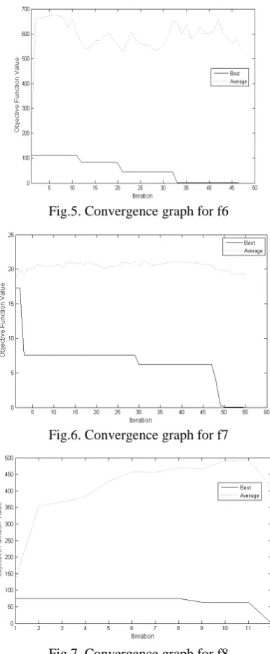
velocity update equations causing displacement of particles in different magnitude and/or direction. In Classical PSO, all particles move towards the weighted mean position of its pbest and gbest of swarm. In GDE-APSO, the particles do not follow its pbest or gbest of swarm always and also they follow different equations in different time (i.e iteration).

From this experimental study, it is seen that GDE-APSO has higher convergence speed in achieving good solutions.

Table 2. Mean and standard deviation of best-error-run, success rate and statistical significance

Table 3. Mean and standard deviation of FEs

Test# GDE-APSO CLPSO

Mean

Std.

Dev. Mean Std. Dev

f1 1078.70 735.97 39491.00 814.93

f2 1741.30 1360.60 100000.00 0.00

f3 1380.70 1239.80 44923.00 716.81

f4 4562.00 4319.60 100000.00 0.00

f5 100000.00 0.00 100000.00 0.00

f6 773.33 597.96 63839.00 28394.00

f7 1359.30 1011.20 43597.00 729.19

f8 1530.00 1074.00 100000.00 0.00

Fig.4. Convergence graph for f5

VII. C

ONCLUSION

(6)

R

EFERENCES

[1] R. C. Eberhart and J. Kennedy(1995):“A new optimizer using

particle swarm theory,” in Proceedings of 6th Symposium on

Micro Machine and Human Science, Nagoya, Japan, pp. 39-43.

[2] J. Kennedy and R.C. Eberhart(1995): “Particle Swarm

Optimization”, in proceedings IEEE Internal Conference on Neural Networks, vol. IV. Piscataway, NJ: IEEE Service Center, pp-1942-1948.

[3] R. Eberhart, P. Simpson and R. Dobbins(1996): Computation

Intelligence PC tools. San Diego, CA, USA: Acedemic Press Professional, Inc.,

[4] M. Clerc, Particle Swarm Optimization. ISTE Publishing

Company, 2006

[5] Y. Shi and R. C. Eberhart(1998):“A modified particle swarm

optimizer,” in proceedings of the IEEE congeres on Evolutionary computation, Piscataway, NJ, pp. 69-73.

[6] Liang, J.J,Qin,A.K, Suganthan P.N., and Baskar,S.(2006)

`Comprehensive Particle Swarm Optimizer for Global Optimization of Multimodal Functions', IEEE Transactions on Evolutionary Computation,Vol.10, No.3, June 2006,pp.~281-295.

[7] C.Li,Y. Liu, A. Zhao,L. Kang and H. Wang (2007):A Fast

Particle Swarm Algorithm with Cauchy Mutation and Natural Selection Strategy,Springer-Verlag,LNCS 4683,pp.334-343.

[8] A. Stacey, M. Jancic and I. Grundy( 2003):Particle swarm

optimization with mutation, in Proc. Congr. Evol. Comput, 2003, pp. 1425-1430, doi: 10.1109/CEC.2003.1299838.

[9] JIAOWei,LIU Guangbin and LIU Dong(2009): Elite Particle

Swarm Optimization with Mutation, Asia Simulation Conference - 7th International Conference on System Simulation and Scienti_c Computing, 2008. ICSC 2008.

[10] Xiaoling Wu and Min Zhong, Particle Swarm Optimization

Based on Power Mutation,ISECS International Colloquium on Computing, Communication, Control, and Management [11] M. Pant, R. Thangaraj and A. Abraham(2008): Particle Swarm

Optimization using Adaptive Mutation, in Proc. 19th International Conference on Database and Expert Systems Application, pp. 519-523

[12] N. Higashi and H. lba(2003):Particle Swarm Optimization with Gaussian Mutation, IEEE Swarm Intelligence Symposium, Indianapolis, pp. 72-79

[13] Jun Tang and Xiaojuan Zhao(2009):Particle Swarm

Optimization with Adaptive Mutation, WASE International Conference on Information Engineering

[14] A.J. Nebro, SMPSO: A New PSO-based Metaheuristic for

Multi-objective Optimization, ieee symposium on Computational intelligence in miulti-criteria decision-making, 2009

[15] Tapas Si, N.D Jana and Jaya Sil (2011) Constrained Function Optimization using PSO with Polynomial Mutation, In:B.K. Panigrahi et al. (Eds.):SEMCCO2011,Part-I,LNCS 7076,pp. 209-216

[16] Tapas Si,N.D Jana and Jaya Sil (2011): Particle Swarm

Optimization with Adaptive Polynomial Mutation, in proc.

World Congress on Information and Communication

Technologies(WICT 2011),Mumbai,India ,pp. 143-147

[17] Nanda Dulal Jana, Tapas Si and Jaya Sil, (2012):Particle Swarm

Optimization with Adaptive Mutation in Particles, 2012 International Congress on Informatics, Environment, Energy and Applications-IEEA 2012 ,IPCSIT vol.38 (2012), IACSIT Press, Singapore

[18] Tapas Si and Nanda Dulal Jana(2012): “Particle Swarm

Optimization with Differential Mutation”, International Journal

of Intelligent Systems Technologies and Applications-Inderscience, to be published.

[19] H. Wang,Y. Liu, S. Zeng,H. Li and C. Li(2007):“ Opposition-based Particle Swarm Optimization with Cauchy Mutation”,

Proceedings of the IEEE Congress on Evolutionary

Computation,pp.4750-4756.

[20] Storn and K. Price: Dierential Evolution -A Simple and Efficient Heuristic for Global Optimization over Continuous Spaces, Journal of Global Optimizationr,Vol. 11 pp 341-359(1997). [21] Koza, J.R.(1992): Genetic Programming: On the Programming

of Computers by Means of Natural Selection,MIT Press.

[22] Poli,R., Langdon,W.B., Holland,O.(2005) :Extending Particle

Swarm Optimization via Genetic Programming,In: Proceedings of EuroGP05

[23] Poli,R., Langdon,W.B., McPhee,N.F (2008):A Field Guide to

Genetic Programming, Available at

http://www.gp-field-guide.org.uk, (With contributions by J.R Koza). GPBIB

[24] Rashid,M. (2010):Combining PSO algorithm and Honey Bee

Food Foraging Behaviour for Solving Multimodal and Dynamic

Optimization Problems,Ph.D Dissertation, Department of

Computer Science, National University of Computer &

Emerging Sciences, Islamabad, Pakistan, Available at

http://prr.hec.gov.pk/Thesis/488S.pdf

[25] O'Neil, M., Ryan, C. (2001) : Grammatical Evolution, IEEE

Trans. Evolutionary Computation 5(4), 349--358

[26] O'Neill, M., Brabazon, A. (2006): Grammatical Differential Evolution, In: International Conference on Artificial Intelligence (ICAI'06) CSEA Press,Las Vegas, Nevada,pp.231-236

[27] X. Yao, Y. Liu and G. Lin, Evolutionary programming made faster, IEEE Transactions on Evolutionary Computation.,vol. 3,pp. 82-102(1999)

[28] N.G Das, (2008): Statistical Methods (Combined Vol) ,Tata

Mcgraw Hill Education Private Limited

A

UTHOR

’

S

P

ROFILE