A New Approaches for Image De-Blurring in Optical Imaging Application Using Derivative Compressed Sensing

(1)

A New Approaches for Image De-Blurring in Optical

Imaging Application Using Derivative Compressed

Sensing

Santosh Mugali, Dr. S. Bhargavi

Abstract - The problem of reconstruction of digital images

from their blurred and noisy measurements is unarguably one of the central problems in imaging sciences. Despite its ill-posed nature, this problem can often be solved in a unique and stable manner, the current presentation focuses on reconstruction of short-exposure optical images measured through atmospheric turbulence. The latter is known to give rise to random aberrations in the optical wave front, which are in turn translated into random variations of the point spread function of the optical system in use. A standard way to track such variations involves using adaptive optics. Thus, for example, the Shack–Hartmann interferometer provides measurements of the optical wave front through sensing its partial derivatives. In such a case, the accuracy of wave front reconstruction is proportional to the number of lens lets used by the interferometer and, hence, to its complexity. Accordingly, in this paper, show how to minimize the above complexity through reducing the number of the lenslets while compensating for under sampling artifacts by means of derivative compressed sensing. Additionally, it provide empirical proof that the above simplification and its associated solution scheme result in image reconstructions, whose quality is comparable to the reconstructions, obtained using conventional measurements of the optical wavefront.

Keywords — Deconvolution, Derivative Compressive

Sampling, Inverse Problem, Shack–Hartmann

Interferometer (SHI).

I. I

NTRODUCTION

Optical imaging is unarguably the field of applied sciences from which the notion of image deconvolution [1] has originated. In particular, in short-exposure turbulent imaging, acquired images are blurred with a PSF, which depends on a spatial distribution of the atmospheric refraction index along the optical path connecting an object of interest and the observer. Due to the effect of turbulence, the above distribution is random and time dependent, which implies that the PSF cannot be known in advance. A standard way to overcome the above limitation is through the use of adaptive optics[2].

The PSF of a short-exposure optical system is determined by its corresponding GPF[3], which can be expressed in a polar form as. P=Aej While, in practice, the amplitude A can be either measured through calibration or computed as a function of the aperture geometry, phase  accounts for turbulence-induced aberrations of the optical wavefront and, hence, is generally unknown at any given experimental time. Fortunately, phaseturns out to be a measurable quantity, and this is where the tools of AO come into play. One of such tools is the Shack–Hartmann interferometer [4],

which allows direct measurement of the gradient of over a predefined grid of spatial coordinates. Subsequently, these measurements are converted into a useful estimate of through numerically solving an associated Poisson equation.

Among some other factors, the accuracy of phase reconstruction by the SHI depends on the size of its sampling grid, which is in turn defined by the number of lenslets composing the wavefront sensor of the interferometer. Unfortunately, the grid size and the complexity of the interferometer tend to increase pro rata which creates an obvious practical limitation. Accordingly, to overcome this problem, we propose to modify the construction of the SHI through reducing the number of its lenslets. Although the advantages of such a simplification are immediate to see, its main shortcoming is obvious as well: The smaller the number of lenslets is, the stronger is the effect of undersampling and aliasing.

These artifacts, however, can be compensated for by subjecting the output of the simplified SHI to the derivative compressed sensing algorithm[5] of As will be shown in the following, DCS is particularly suitable for reconstruction of from incomplete measurements of its partial derivatives. The resulting estimates of can be subsequently combined with to yield an estimate of PSF , which can in turn be used by a deconvolution algorithm[6-7]. Thus, the proposed method for estimation of PSF and subsequent deconvolution of can be regarded as a hybrid deconvolution technique, which comes to simplify the design and complexity of the SHI, on one hand, and to make the process of reconstruction of optical images as automatic as possible, on the other hand.

II. S

HACK

–

H

ARTMANN

I

NTERFEROMETER

As it was mentioned earlier in this paper, the SHI can be used to measure the gradient of∇∅(x,y) the GPF phase∅ (x,y) ,from which its values can be subsequently inferred. A standard approach to this reconstruction problem is to assume the unknown phase∅ (x,y) to be expandable in terms of some basis Functions{ }∞ _{, as shown in the} following.

∅(x,y)=∑∞ _{( , )} ₍₁₎

where the representation coefficients

{ }∞ _{are supposed to be unique and stably computable.} Note that, in this case, the data of { }∞ uniquely identify∅ (x,y) whereas the coefficients{ }∞ can be estimated due to the linearity of (6) that suggests

∇∅(x,y)=∑∞ ∇ ( , ) (2)

(2)

functions defined over the unit disk in .Zernike polynomials can be subdivided in two subsets of the even and odd Zernike polynomials, which possess closed-form analytical definitions as given by

( , )= ( )cos(mφ) (3)

( , )= ( ) sin(mφ) (4)

where and are non negative integers with n≥m,0≤<2 is the azimuthal angle, and 0≤ ≤ 1 is the radial distance.The radial polynomials in (3) and (4) are defined as

( ) = ∑ _!( ) (_!( )

( ))!

/ ₍₅₎

Note that, since the Zernike polynomials are defined using polar coordinates, it makes sense to reexpress the phase andits gradient in the polar coordinate system as well (technically,this would amount to replacing x and y in (6) and (7) by andφ, respectively). Moreover, due to the property of the Zernike polynomials to be an orthonormal basis, the representation coefficients in (6) and (7) can be computed by orthogonal projection, namely

= ∬ ∅( , ) ( , ) . (6)

In practice, however,∅(x,y) is unknown; therefore, the coefficients{ }∞ need to be estimated by other means. Thus, in the case of the SHI, the coefficients can be estimated from a finite set of discrete measurements of∇∅ (x,y).

Fig.1. Example of a 10* 10 SHI array on a circular aperture. The shading indicates those blocks (i.e., lenslets)

that are rendered active.

The main function of the SHI is to acquire discrete measurements of ∇∅ by means of linearization. The linearization takes advantage of subdividing a (circular) aperture into rectangular blocks with their sides formed by a uniform rectangular lattice. An example of such a subdivision is shown in Fig. 1 for the case of a 10 *10 lattice grid. In general, the grid is assumed to be sufficiently fine to approximate by a linear function over the extent of a single block. This results in a piecewise linear approximation of, whose accuracy asymptotically improves when the lattice size goes to infinity. Formally, let be a circular aperture of radius D and S={(x,y) be a square subset of such that . Then, for each polar coordinate and an grid of square blocks of size, the phase can be expressed as

∅(x,y)≈ax+by+c (7)

for all (x,y) in a neighborhood of (ρcosφ,ρsin ).The approximation in (7) suggests that

∇∅(x,y) =( , ) (8)

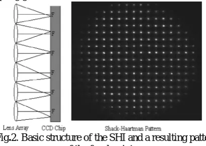
where(. ) denotes matrix transposition.While in (7) can be derived from boundary conditions, coefficients and should be determined through direct measurements. To this end, the SHI is endowed with an array of small focusing lenses (i.e., lenslets), which are supported over each of the square blocks of the discrete grid, thereby forming a wavefront sensor. In the absence of phase aberrations, the focal points of the lenslets are spatially identified and registered using a high-resolution CCD detector, whose imaging plane is aligned with the focal plane of the sensor. Then, when the wavefront gets distorted by atmospheric turbulence, the focal points are dislocated toward new spatial positions, which can also be pinpointed by the same detector. The resulting displacements can be measured and subsequently related to the values of ∇∅ at corresponding points of the sampling grid.

Fig.2. Basic structure of the SHI and a resulting pattern of the focal points.

To explain how the given procedure can be performed, additional notations are in order. LetΩ denote a finite set of spatial coordinates defined according to

Ω = _, Ω

,= + + , = 0,1,2 … … . . − 1

= + + , = 0,1,2 … . . − 1

And + ≤ } (9) The

setΩ can be thought of as a set of the spatial coordinates of the geometric centers of the SHI lenslets, which are restricted to the domain of its aperture Ω. Under the assumption of (7), one can then show that the focal displacement ∆(x,y)=[ ∆ ( , ), ∆ ( , )] measured at some(x,y) Ω is related to the value of ∇∅ (x,y) according to

∇∅(x,y)1/F∆∅(x,y)(x,y)Ω (10) where F is the focal distance of the wavefront lenslets. An example of the given measurement setup is depicted in Fig. 2. whose definition is unique and stable as long as the row rank of Z is greater or equal L+1 to (hence, suggesting that 2M ≥L+1). Having estimated, phase can be

approximated as

(3)

III. D

ERIVATIVE

C

OMPRESSED

S

ENSING

Let the partial derivatives of evaluated at the points of set be column-stacked into vectors and of length M=#Ω In what follows, the partial derivatives and are assumed to be sparsely representable by an orthonormal basis in . Representing such a basis by an MxM unitary matrix W, the given assumption suggests the existence of two sparse vectors cxand cysuch that fx=Wcx

and fy=Wcy. In the experimental studies reported in this

paper, matrix W is constructed using the nearly symmetric orthogonal wavelets of Daubechies having five vanishing moments[10] .

The proposed simplification of the SHI amounts to reducing the number of wavefront lenslets. Formally, such a reduction can be described by two nM subsampling matricesxandy, where n<M. Specifically, let bx:=xfx

and by:=yfybe incomplete (partial) observations of fxand

fy, respectively. Then, based on the theoretical guarantees

of CCS, the vectors fxand fyof the partial derivatives of ø

can be approximatedbyW ∗and Wcy*, respectively, where

cx* and ∗are obtained as

∗₌ _ _{ __{c W}  _{- b}

x +x 1}

(12) ∗₌ _ _{ __{c W} _{- b}

y +y 1} (13)

for somex,y >0. Moreover, in the case when x

=y:=,computing the given estimates can be combined

into a single optimization problem. Specifically, let , c =[cx ,cy]T,b =[bx,by]T, and A = diag { xW ,yW}

R2n x2 M. Then

c*=arg ′ ={ A ′−  + ′1}. (14)

In this form, problem is identical to in which case it can be solved by a variety of available tools of convex optimization [13].

The DCS algorithm augments CCS by subjecting the minimization to an additional constraint that stems from the fact that [5]

∅₌ ∅ ₍₁₅₎

which is valid for all twice continuously differentiable functions ∅. Thus, in the discrete setting, the given condition can be expressed using two partial differences matrices and DxDy, in which case it reads

Dxfy= Dyfx. (16)

To further simplify the notations, let Txand Ty be two

coordinate-projection matrices, which map the composite vector into cx and cy according to Txc= cx and Tyc= cy,

respectively. Then, (19) can be reexpressed in terms of c as

DyWTxc= DxWTyc (17)

Or, equivalently

Bc=0 (18)

Where B:= DyWTx−DxWTy. Consequently, with the

addition of the cross-derivative constraint, DCS solves the constrained minimization problem given by

c*=arg ′ { A ′−  + ′1}, s.t. B ′=0. (19)

A solution to () can be found, for instance, by means of the Bregman algorithm, in which case is obtained as a stationary point of the sequence of iterations produced by

( )_{= arg}

′ X{ A ′− 

+ ′_

1+

_

B ′₊ ( )_ _}

( )₌ ( )₊_ ( ) ₍₂₁₎ where p(t)is a vector of Bregman variables and> 0is a user-defined parameter2. Note that the c-update step in (21) has the format of a standard basis pursuit denoising problem, which can be solved by a variety of optimization methods. In this paper, we used the FISTA algorithm in due to the simplicity of its implementation as well as for its remarkable convergence properties.

It should be noted that the algorithm does not require explicitly defining the matrices A and B. Only the operations of multiplication by these matrices and their transposes need to be known, which can be implemented in an implicit and computationally efficient manner.

Once an optimal c* is recovered, it can be used to estimate the noise-free versions of fxand fyas WTxc*and

WTyc *

, respectively. These estimates can be subsequently passed on to the fitting procedure in Section III to recover the values of ∅, which, in combination with a known aperture function A, provide an estimate of the PSF I as an inverse discrete Fourier transform of the autocorrelation of P=Ae3ø . Algorithm 1 below summarizes our method of estimation of the PSF.

Algorithm 1: PSF estimation via DCS 1) Data: bx, by, and>0

2) Initialization: For a given transform matrix W and matrices/operators x,y, Dx, Dy, Tx, and Ty, preset the

procedures of multiplication by A, AT, B, and BT.

3) Phase recovery: Starting with an arbitrary c(0) and c(0)=0, iterate (21) until convergence to result in an optimal c*. Use the estimated (full) partial derivatives WTxc

*

and WTyc*to recover the values of∅overΩ.

4) PSF estimation: Using a known aperture function A, compute the inverse Fourier transform of P=Ae3øto result in a corresponding ASF h. Estimate the PSF i as i=h2.

The estimated PSF can be used to recover the original image u from v through the process of deconvolution, as explained in the section that follows.

IV. D

ECONVOLUTION

The acquisition model (1) can be rewritten in an equivalent operator form as given by

V= H{u}+v (22)

where H denote the operator of convolution with the estimated PSF i. Note that, in this case, the noise term v accounts for both measurement noise as well as the inaccuracies related to estimation error in i.The deconvolution problem of finding a useful approximation of u given its distorted measurement v can be addressed in many way, using a multitude of different techniques .In this paper, we use the ROF model and recover a regularized approximation of the original image u as

(4)

variation (TV) semi-norm of The minimization problem in (23) can be solved using a magnitude of possible approaches. One particularly efficient way to solve is to substitute a direct minimization of the cost function in (23) by recursively minimizing a sequence of its local quadratic majorizers. In this case, the optimal solution * can be obtained as the stationary point of a sequence of intermediate solutions produced by

( )₌ ₊ ∗ ₋ ( )

( )_{= arg} 1

2H{u}– 

2

2 +  TV (24)

where H is the adjoint of and is chosen to satisfy. In this paper, the TV denoising at the second step of (24) has been performed using the fixed-point algorithm in [11]. The convergence of (24) can be further improved by using the same FISTA algorithm[18]in The resulting procedure is summarized in Algorithm 2.

Algorithm 2: TV deconvolution using FISTA

1) Initialize: Select an initial value u(0);set y(0) =u(0) and

(0)

=1

2) Repeat until convergence:

 ( )₌ ₊ ∗_{{ −} ( ) _}

 ( )_{= arg} _{ __{H{u} –} _ ₊ _{ }_TV}

 ( )_{= 0.5(1 + 1 + 4(}_( )₎2₎

 ( ) ₌ ( )₊ ( )

( ) ( ( )− ( ))

In summary, Algorithms 1 and 2 represent the essence of the proposed algorithm for hybrid deconvolution of short-exposure optical images. The next section provides experimental results that further support the value and applicability of the proposed methodology.

V. R

ESULTS

To demonstrate the viability of the proposed approach, its performance has been compared against reference methods. The first reference method used a dense sampling (DS) of the phase (as it would have been the case with a conventional design of the SHI), thereby eliminating the need for a CS-based phase Reconstruction. The resulting method is referred below to as the DS approach. Second, to assess the importance of incorporation of the cross-derivative constraints, we have used both CCS and DCS for phase recovery. In what follows, comparative results for phase estimation and subsequent deconvolution are provided for all the given methods.

A. Image Deconvolution:

The phase estimates obtained using the CCS and DCS-based methods for were combined with the aperture function to result in their respective estimates of the PSF . These estimates were subsequently used to deconvolve a

number of test images such as “Satellite,” “Saturn,” “Moon,” and “Galaxy.” All the test images

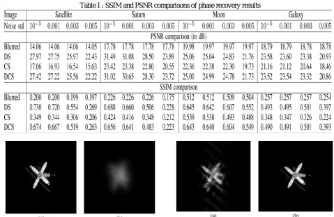
Table I : SSIM and PSNR comparisons of phase recovery results

Fig.3. (a) Satellite image and (b) its blurred and noisy version

Fig.4. (a) Image estimate obtained with the CCS-based method for phaserecovery (SSIM=0.781) . (b) Image estimate obtained with the DCS-based method for phase

(5)

contamination with additive Gaussian noise of different levels, which is controlled by the variance of noise

distribution. As an example, the “Satellite” image along

with its blurred and noisy version are shown in Fig. 3(a) and (b), respectively. Using the PSF estimates, the deconvolution was carried out using the method detailed in [11]. For the sake of comparison, the deconvolution was also performed using the PSF recovered from DS of∅.Note that this reconstruction is expected to have the best accuracy since it neither involves undersampling nor requires a CS-based phase estimation. All the deconvolved images have been compared with their original counterparts in terms of PSNR as well as of the structural similarity index (SSIM) which is believed to be a better indicator of perceptual image quality The resulting values of the comparison metrics are summarized in Table I, whereas the deconvolution results produced by the CCS-and DCS-based methods are shown in Fig. 4

Fig.5. (a) Image estimate obtained with the CCS-based method for phase recovery (SSIM=0.732) . (b) Image estimate obtained with the DCS-based method for phase

recovery (SSIM =0.886) where the noise model is assumed to be Poisson.

The given results demonstrate the importance of accurate phase recovery, where even a relatively small phase error can have a dramatic effect on the quality of image deconvolution. Under such conditions, the proposed method produces image reconstructions of a superior quality, as compared with the case of CCS. Moreover, comparing the results in Table I, one can see that DS only slightly outperforms DCS in terms of PSNR and

SSIM, whereas in many practical cases, the difference between the performances of these methods are hard to detect visually. Finally, the results of CCS-based and DCS-based image reconstructions for the case of Poisson noise contamination are shown in Fig. 5. A close comparison of these results reveals a noticeable degradation in the performance of the CCS-based algorithm, whereas the DCS-based results are virtually indistinguishable from those obtained in the Gaussian case.

V. D

ISCUSSION AND

C

ONCLUSION

In this paper, the applicability of DCS to the problem of reconstruction of optical images has been demonstrated. It was shown that, in the presence of atmospheric turbulence, the phase of GPF is a random function, which needs to be measured using AO. To simplify the complexity of the latter, a CS-based approach has been proposed. As opposed to CCS, however, the proposed method performs

phase reconstruction subject to an additional constraint, which stems from the property of to be a potential field. The DCS algorithm has been shown to yield phase estimates of substantially better quality as compared with the case of CCS.

In this paper, our main focus has been on simplifying the structure of the SHI through reducing the number of its wavefront lenslets while compensating for the effect of undersampling by means of DCS. The solution was computed using the Bregman algorithm, which provides a computationally efficient framework to carry out the constrained phase recovery. Moreover, the resulting phase estimates were used to recover their associated PSF, which was subsequently used for image deconvolution. It was shown that the DCS-based estimation of with results in image reconstructions of the quality comparable to that of DS while substantially outperforming the results obtained with CCS.

While the proposed method offers a practical solution to the problem of phase estimation in AO, some interesting questions about the theoretical aspects of DCS still lay open. In particular, the question of theoretical performance of CS in the presence of side information on the source signal needs to be addressed through future research. For practical purpose one can also take benefit of this algorithm to modify the SHI. Instead of working with the measurements of the phase gradient, their linear combination can be used, e.g., Bernoulli weights. The resulting sensing basis might have smaller coherence with respect to the basis of wavelets, thereby offering the possibility of more accurate and stable reconstruction.

ACKNOWLEDGMENT

The authors would like to thank our college staff and friends for help full comments.

R

EFERENCES

[1] J. Yang, J. Wright, T. S. Huang, and Y. Ma, “Image super

-resolution via sparse representation,” IEEE Trans. Image Process., vol. 19, no.11, pp. 2861–2873, Nov. 2010.

[2] M. J. Cullum, Adaptive Optics. Garching, Germany: Eur. SouthernObservatory, 1996.

[3] D. L. Fried, “Statistics of a geometric representation of wavefront distortion,”J. Opt. Soc. Amer., vol. 55, no. 11, pp.

1427–1431, 1965.

[4] D. Dayton, B. Pierson, B. Spielbusch, and J. Gonglewski,

“Atmospheric structure function measurements with a Shack–

Hartmannwave-front sensor,” J. Math. Imag. Vis., vol. 20, pp.

89–97, 2004.

[5] M. Hosseini and O. Michailovich, “Derivative compressive

sampling with application to phase unwrapping,” in Proc. EUSIPCO, Glasgow,U.K., Aug. 2009..

[6] J. A. Cadzow, “Blind deconvolution via cumulant extrema,” IEEE Signal Process. Mag., vol. 13, no. 3, pp. 24–42, May 1996. [7] D. Kundur and D. Hatzinakos, “Blind image deconvolution,” IEEE Signal Process. Mag., vol. 13, no. 3, pp. 43–64, May 1996. [8] R. G. Lane and M. Tallon, “Wave-front reconstruction using a Shack–Hartmann sensor,”Appl. Opt., vol. 31, pp. 6902–6908, 1992..

[9] V. Torre, T. Poggio, and C. Koch, “Computational vision and regularizationtheory,”Nature, vol. 317, pp. 314–319, Sep. 1985. [10] I. Daubechies, Ten Lectures on Wavelets. Philadelphia, PA:

(6)

[11] A. Chambolle, “An algorithm for total variation minimization and applications,”J. Math. Imag. Vis., vol. 20, no. 1, pp. 89–97, Jan. 2004.

[12] T. Goldstein and S. Osher, “The split bregman method for l1

-regularized problems,”SIAM J. Imag. Sci., vol. 2, no. 2, pp.

323–343, 2009.

[13] D. L. Donoho and Y. Tsaig, “Fast solution of -norm

minimization problems when the solution may be sparse,” 2006.

[14] L. He, A. Marquina, and S. Osher, “Blind deconvolution using tv regularization and bregman iteration,” Int. J. Imag. Syst. Technol., vol. 15, no. 1, pp. 74–83, 2005.

[15] O. Michailovich and A. Tannenbaum, “Blind deconvolution

ofmedical ultrasound images: Parametric inverse filtering

approach,” IEEE Trans. Image Process., vol. 16, no. 12, pp.

3005–3019, Dec. 2007.

[16] W. H. Richardson, “Bayesian-based iterative method of image

restoration,”J. Opt. Soc. Amer. A, vol. 62, no. 1, pp. 55–59, 1972.

[17] L. B. Lucy, “An iterative technique for the rectification of observed distributions,”Astron. J., vol. 79, no. 6, pp. 745–754, Jun. 1974

[18] I. Daubechies, M. Defrise, and C. D. Mol, “An iterative

thresholding algorithm for linear inverse problems with a

sparsity constraint,”Commun. Pure Appl. Math., vol. 57, pp.

1413–1457, 2004.

A

UTHOR

’

S

P

ROFILE

Santosh Mugali

is presently pursuing final semester M.Tech in Signal Processing at SJCIT Chickballapur. (Visvesvaraya Technological University Belagum) he received degree B.E in Electronics and communication From VTU Belagum his areas of interest are Signal Processing, Image Processing, Low Power VLSI, DSP algorithm And Architecture.