Uncertainties due to Fuel Heating Value and Burner Efficiency on Performance Functions of Turbofan Engines Using Monte Carlo Simulation

Please cite this article as: M. Gorji, A. Kazemi, D. D. Ganji, Uncertainties due to Fuel HeatingValue and Burner Efficiency on Performance Functions of Turbofan Engines Using Monte Carlo Simulation. International Journal of Engineering (IJE) Transactions A: Basics, Vol. 27, No. 7, (2014): 1139-1148

International Journal of Engineering

J o u r n a l H o m e p a g e : w w w . i j e . i r

Uncertainties due to Fuel Heating

Value and Burner Efficiency on Performance

Functions of Turbofan Engines Using Monte Carlo Simulation

M. Gorji, A. Kazemi*, D. D. Ganji

Department of Mechanical Engineering, Babol Noshirvani University of Technology, Babol, Iran

P A P E R I N F O

Paper history:

Received 26 May 2013

received in revised form 22 September 2013 Accepted 07 November 2013

Keywords: Monte Carlo Uncertainty Turbofan Engine

A B S T R A C T

In this paper, the impacts of the uncertainty of fuel heating value as well as the burner efficiency on performance functions of a turbofan engine are studied. The mean value and variance curves for thrust, thrust specific fuel consumption as well as propulsive, thermal and overall efficiencies are drawn and analyzed, considering the aforementioned uncertainties based on various Mach numbers at a number of flying altitudes in order to yield a more accurate prediction of values of performance functions. The results of this study can be of essential significance for an optimal and robust design of turbofan engines. This study is done employing Monte Carlo Simulation method which is a probabilistic analysis method.

doi: 10.5829/idosi.ije.2014.27.07a.16

NOMENCLATURE

0

a Velocity of sound at inlet(m/s) p Pressure ratio

P

C Specific heat at constant pressure(kJ/kg K) t Temperature ratio

F Thrust(N) pf Density (kg/m3₎

0

m& Mass flow rate(kg/s) t Fan pressure ratio

f

m& Mass fuel rate(kg/s) a Bypass ratio

0

M Flight Mach number e Polytropic efficiency

h Flight altitude(Km) hmH High pressure spool mechanical efficiency

PR

h Heating value(kJ/kg) hmL Low pressure spool mechanical efficiency

R Gas constant(J/kg/s) Subscripts

0

m

F & Specific thrust (N/kg/s) cH High pressure compressor

S Thrust specific fuel consumption(mg/s)/N cL Low pressure compressor

4

t

T Turbine inlet temperature(K) tH High pressure turbine

T Temperature(K) tL Low pressure turbine

V Velocity(m/s) f Fan

g _{Ratio of specific heats} b Burner

T

h Thermal efficiency n Nozzle

P

h Propulsive efficiency fn Fan nozzle

o

h Overall efficiency d Diffuser

1. INTRODUCTION

Uncertainty refers to whatever we suffer the lack of information of and, in fact, results from our incomplete knowledge of a phenomenon. Since uncertainty rises from our incomplete knowledge which leaves us unable to talk about the certain occurrence of a phenomenon, we talk about the probability of its occurrence. Uncertainty and probability are terms which are frequently used together. There are quite a significant number of uncertainties in engineering problems. In engineering problems, in addition to our improper knowledge of the system including imprecise measurements of parameters and changes in parameters due to a number of reasons such as time and disturbance which in turn causes uncertainty, another factor causing uncertainty is the mathematical model employed for system analysis. This type of uncertainty might be due to the simplifications of the model.

There are plenty of uncertainties in engineering problems. In vehicle design, there is a lack of proper information about the number of passengers and the weight the vehicle has to practically tolerate. The only thing we can do is to predict the occurrence within a range. The imposed load on the buildings is never precisely predictable and it is only possible to make estimations based on previous knowledge. There, also uncertainties in all parameters which are usually considered constant in designing process. A crucially important point to remember is that if a designed device exhibits a fully desirable and optimal performance within a certain space, it may fail to exhibit such optimal performance in case of uncertainty occurrence. In fact, this undesirable performance may cause a significant increase in the system risk. A number of such cases can be found in references [1] and [2].

Regarding the study of uncertainties, Papadrakakis employed robust design methods in order to achieve an optimal multi-objective design for a six-story building [3]. The elasticity module, imposed loads, and geometrical dimensions of parameters were probabilistic uncertainties. The two functions of weight of structure in certain space, and the variance of the system’s response to the uncertainties in the parameters of the system were chosen for optimization. In 2005, Papadrakakis employed probabilistic analysis for building design and three-dimensional truss [4]. He also used probabilistic analysis to yield an optimal design of a three-dimensional truss tower with the height of 128 meters and a square base area of 17.07 m2 _{[5]. In 2008,}

Kumar used probabilistic analysis for the optimal design of compressor blade [6]. The design variable in that study was blade profile and the target functions were minimization of mean and variance of compressor pressure loss. Imprecision in manufacturing the blade was considered the probabilistic uncertainty. It has also

been shown in this study that the optimal points achieved through certain analysis of a system with uncertainties may not be trusted. In 2009, Lalonde studied the capabilities of Multi-objective optimization algorithms in solving problems with uncertainty [7].

The performance functions of turbofan engines are investigated in many references [8-13] in which the effects of uncertainties were not considered.

In this paper, the impacts of the uncertainty of fuel heating value as well as the burner efficiency in a turbofan engine are studied in order to yield a more accurate prediction of values of performance functions. This study is done employing Monte Carlo Simulation method which is a probabilistic analysis method. In order to resist uncertainties, the design model should be in such way that makes the system robust against the uncertainties.

2. TURBOFAN ENGINE

Figure 1 illustrates a turbofan engine. Turbines and compressors are divided into Low Pressure and High Pressure sections. The High Pressure turbine turns the High Pressure compressor via High Pressure spool, and the Low Pressure turbine turns the Low Pressure compressor via Low pressure spool. The mass flow passing through the engine core and fan are m&_Cand m&_F

respectively. The ratio of mass flow through fan to mass flow through engine core is introduced as bypass ratio and is shown by α. The Sea-Level static conditions are considered as the design point conditions for gas turbine variables [8-9]. The assumed condition in turbofan engine is the one in which the inlets at High-Pressure turbine as well as Low-Pressure turbine experience choking. Also, the nozzle section areas are considered constant at the inlet of High-Pressure and Low-Pressure turbines. This type of turbines is known as Fixed Area Turbine (FAT).

This assumption is valid within a wide performance range of gas turbine engines [8, 10]. Also, based on the assumptions of reference [8], the pressure ratios of combustion chamber, exit nozzle, and bypass exit nozzle as well as other components efficiencies such as compressor and turbine do not deviate from design point values. Effects of turbine cooling and leakage are neglected. Also, the turbine power is not used to run the side components. Gas in the both upstream and downstream of combustion chamber is also considered perfectly . The inlet flight Mach number and flight altitude are the independent input variables. The most important output parameters which are considered as performance functions in the turbofan engine are thrust, thrust specific fuel consumption, and propulsive, efficiency, and overall efficiency [10-12]. The aforementioned functions in turbofan engine come in the form of Equations (1) to (6) (8-9):

÷÷ ø ö çç è æ = 0 0 _mF

m F & & (1) ÷÷ ø ö çç è

æ _{- +}

-´ + + ú û ù -´ ê ë

é _{+ - + +}

+ = c c c t P P a V T T M a V a P P a V R T T R f M a V f a m F g a a g a 19 0 0 19 0 19 0 0 19 0 9 0 0 9 0 9 0 0 9 0 / 1 / / 1 / 1 / / ) 1 ( ) 1 ( 1 1 o & (2) 0 / ) 1

( F m

f S & a + = ₍₃₎ ( ) [ ]

( ) ( ) 2

0 2 0 19 2 0 9 0 0 19 0 9 0 ) 1 ( / / ) 1 ( ) 1 ( / / ) 1 ( 2 M a V a V f M a V a V f M P a a a a h + -+ + + -+ + = ₍₄₎

[

]

PR

T a f V a _2fhV a M

) 1 ( ) / ( ) / )( 1 ( 2 0 2 0 19 2 0 9 2

0 a a

h = + + - + (5)

T P o h h

h = (6)

The engine reference values (the design point conditions) at sea level and at zero Mach number are as follows: 99 . 0 96 . 0 997 . 0 9915 . 0 8815 . 0 8512 . 0 99 . 0 9636 . 0 7262 . 0 9625 . 0 7580 . 0 239 . 1 004 . 1 3 . 1 4 . 1 42800 sec 760 1890 8 4 2 8 max 0 4 = = = = = = = = = = = = = = = = = = = = = = = = = d fn n b mL mH f cL cH b tL tL tH tH pt pc t c PR t cH cL f C C kg kJ h kg m K T p p p p h h h h h h h t h t g g p p p a &

The compressor pressure ratio is limited at 32. Also, the maximum exit temperatures of combustion chamber and high pressure compressor are 1890 and 920 o_K

respectively. In this case, bypass ratio, fan and compressor pressure ratio, combustion chamber and compressor exit temperature ratios, and the corrected mass flow passing through compressor and fan are controlled by the engine controller. The performance

functions of such a turbofan engine have been thoroughly studied in [13].

3. PROBABILITY DENSITY FUNCTION (PDF)

Density functions are mostly used by engineers to describe physical systems. If fX

( )

x is the probability density function which is used to describe the probable distribution of a random variable such as X, the probability of occurrence of the process X will be between the two values of a and b which is equal to the integral of the area covered by density function between the points of a and b. The probability density function is of the following characteristics:

( )

( ) ( )

( )7.3 ( ) ( ) . ) 1 . 7 (

ò

ò

= £ £ = ³ ¥ ¥ -b a X X X dx x f b X a P 1, dx x f 7.2 0, x f (7)

The probability density function provides a simple description of the related probabilities of a random variable. In Equation (7), P

(

a£X£b

)

is the probability of occurrence of a condition in which the random variable X is of a value between a and b. according to Equations (7.1) and (7.2), this probability always has a value between 0 and 1

(

0£P

(

a£X£b

)

£1

)

. During a random process, the value of probability density function for Xs which do not occur is zero [14].

4. CUMULATIVE DISTRIBUTION FUNCTION (CDF)

Another method for showing the related probabilities of random variable is to use cumulative distribution function

(

FX

( )

x

)

. This function is defined as follows:

( ) ( )

ò

( ) . ¥ -= £ = x

Xudu f x X P x F (8)

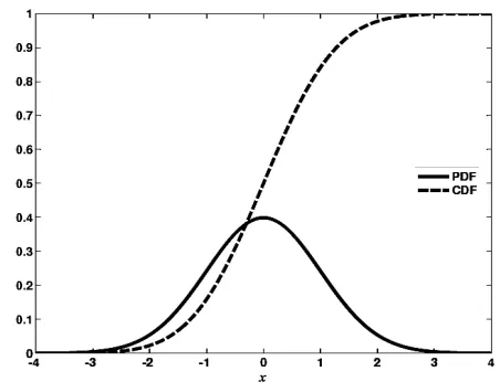
Figure 2 illustrates the curves for cumulative distribution function and probability density function for the random variable X.

( )

ïî ï í

ì _{£ £}

-=

otherwise 0

d X c d c

1 x

f_X (9)

where c and d are upper and lower limits respectively. For a number of variables, Gaussian distribution might be a good estimate of probability their occurrence. A Gaussian cumulative distribution function is shown as follows:

( ) -¥< <+¥

ú ú û ù ê

ê ë é

÷ ø ö ç è

æ

-î

í ì

= , X

σ μ X 2 1 exp 2π σ

1 x f

2

X (10)

where

μ

and

σ

are mean and variance of the probabilistic variable x. Gaussian distribution function is symmetric about the value of mean. Beta distribution function is defined as follows:

( )

ïî ï í

ì _{< <}

=

otherwise 0

X X)

-(1 X b) B(a,

1 x

f_X a-1 b-1 0 1 (11)

where B(a, b) is beta function and a and b are shaping coefficients. The shape of cumulative function is dependent on a and b, and varies accordingly.

5. MEAN AND VARIANCE

There are two quantities normally used to define the probabilistic distribution of a random variable such as X. Mean is the value of mode or median of probabilistic distribution and variance is the scatteredness or changeability in distribution [14]. If we assume that X is a random variable with the probabilistic density functionf_X

( )

x , then the mean of X is shown by

m

or E[X], and is defined as follows:

[ ]

¥

_ò

( )

¥ -=

=EX xf xdx

μ X

(12)

Variance X which is shown by

s

2or V

[ ]

X is equal to the following:

[ ]

_ò

( ) ( )

_ò

¥ ( )

¥ -¥

¥

-=

-=

= 2

X 2 X

2

2 _{VX x μ f xdx x f xdx μ}

σ (13)

For discrete cases of these equations, the above integrals are shown as follows:

[ ]

å

= »

N

1 i

i

x N 1 X

E (14)

[ ]

_å

( [ ])

= -»

N

1 i

2

i EX

x 1 N

1 X

V ₍₁₅₎

where

x

_i is the ith sample and N is the number of total

samples. For continuous systems, the Equations (12) and (13) have to be solved; this is impossible to do due to the complexity of the integrals. Therefore, numerical simulation methods are employed to yield estimations. One of the most frequently used methods is the Monte Carlo method [15-17]. Employing this method, the integrals of the Equations (12) and (13) are estimated by Equations (14) and (15).

6. MONTE CARLO METHOD

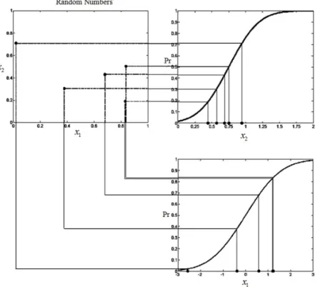
Simply put, Monte Carlo method is a numerical simulation method using random sampling from the uncertain parameters space. This method is based on a random generation of numbers between zero and one. Once the random generation of numbers between zero and one has been done, random samples of uncertain parameters are generated based on their cumulative distribution, and then the system is simulated as per each randomly generated sample. Subsequently, it will be possible to calculate the probability of each occurrence using numerical methods. In Monte Carlo method, sample is an n-dimensional vector like

(x₁,x₂, ,x_n)

X= _K where n is the number of uncertain parameters. Figure 3 illustrates the simulation process for the parameters x1 and x2 using random generation of numbers and desired distribution. As it can be seen, first, a series of random numbers belonging to the range

[ ]

0,1 Î n

l (in this example n=2) is generated. Each of these numbers represents the probability of occurrence of the considered uncertain parameter. Then, the value of each parameter is calculated using its cumulative distribution function, and the vector of uncertain parameters is formed.

Figure 3. Monte Carlo simulation.

Figure 4. Probability Density Function for burner efficiency.

7. STUDY OF THE UNCERTAINTIES OF TURBOFAN ENGINES USING MONTE CARLO SIMULATION

The aim of this section is to study the impact of changes in uncertain parameters on the functional graphs of the system. Among the existing constant parameters in turbofan engines, the impacts of changes in the burner efficiency as well as the heating value of fuel are studied. The assumption of burner efficiency uncertainty is due to a relative decrease in this efficiency as a result of the combustion process in the engine. Furthermore, since the quality of the fuel production is subject to change in different parts of the world, the heating value of the fuel cannot be constant. Thus, it would be valid to assume this quantity as an

uncertain parameter. The other constant parameters mentioned in section 2 are certain due to careful maintenance of the aircraft. The next step is to yield the curves of probability density function (PDF) as well as cumulative distribution function (CDF) according to what has been mentioned in sections 4 and 5. Then, the variance and mean of performance functions are calculated for various samples generated by cumulative distribution function and the correspondent curves are drawn. A detailed account of this process will follow.

7. 1. Probability Density Function and Cumulative Distribution Function of Uncertain Parameters

As it was mentioned earlier, burner efficiency and fuel heating value are chosen as uncertain parameters. Now, according to what has been presented in section 4 in terms of Equations (7), it is possible to yield Probability Density Function of the above-mentioned parameters. First, burner efficiency is studied. Assuming that combustion chamber efficiency decreases from 99% to 96% through a linear distribution, the area under PDF forms a triangle. According to Equation (7.2), it is possible to determine the height of the triangle (in Figure 4).

( )

03 . 0

2 1 2

96 . 0 99 .

0 - _{= ® =}

´

y y

And the equation of the line passing through the points a and b is achieved as follows:

( )0.03 ( 0.96) 2

)

(x = ₂ x

-F ₍₁₆₎

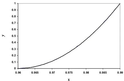
Now, according to Equation (8), Cumulative Distribution Function is achieved as follows:

( ) ( )

96 . 0 03 . 0

03 . 0

96 . 0 96

. 0 03 . 0

2 2

96 . 0

2

+ = ®

÷ ø ö ç è æ -= -=

ò

y x

x du u y

x

(17)

When analyzing fuel heating value, it is assumed that this parameter is of a Gaussian distribution within the range of 41800kJ kg to 43800kJ kg with the maximum value of F(x) in 42800kJ kg. Gaussian distribution which is presented in Equation (10) yields a desirable distribution having m=42800 and s=224. Figure 6 illustrates this distribution.

In order to achieve Cumulative Distribution Function, Matlab norminv operation is employed. This operation with the structure of X=norminv (P, mu, sigma) will take X=norminv (P,42800,224) for the mentioned problem. This operation generates values between 41800kJ kg and 43800kJ kg per each random number between 0 and 1 assigned to P. Figure 7 illustrates the Cumulative Distribution Function for fuel

PDF for burner efficiency

0 10 20 30 40 50 60 70 80

0.955 0.96 0.965 0.97 0.975 0.98 0.985 0.99 0.995

x

F

(x)

a=(0.96,0)

heating value. The interesting point in this curve is that due to the high slope of the curve for x values near

kg kJ

42800 , a large portion of the randomly generated numbers between 0 and 1, for instance between 0.3 and 0.8, take values near 42800kJ kg. Now, as the Cumulative Distribution Function curve for uncertain parameters has been achieved, it will be possible to determine the values of these parameters through generating random numbers between 0 and 1.

7. 2. The Uncertainties Impact on Performance Functions… .Figures 8 through 17 illustrate means and variances of performance functions including thrust, specific fuel consumption, thermal, thrust, and overall efficiencies based on various Mach numbers and flight altitudes. These curves are drawn based on N random points of each uncertain parameter. For instance, in N=150, 150 random points between zero and one are generated, and then the values of burner efficiencies are achieved based on its CDF curve from Figure 5.

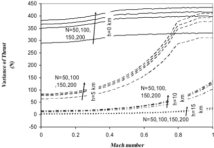
Likewise, by generating another 150 random points, 150 equivalents of fuel heating value are achieved from Figure 7. Mean and variance of performance functions have been achieved for 50, 100, 150, and 200 points, as mentioned above. As well, these curves have been drawn for the nominal values of the uncertain parameters. Figure 8 illustrates the mean of thrust for various Mach numbers at different altitudes. As it can be seen, at all altitudes, the nominal values and the values achieved through N different points match each other. Figure 9 illustrates thrust variance. As it can be seen, as altitude increases variance significantly decreases and nearly reaches zero at 15 km. Variance increases as the Mach number increases at various altitudes. This increase reaches a significant point at h= 5Km. Also, at a certain altitude, as N increases variance increases accordingly. Through analyzing Figures 8 and 9, it might be concluded that the assumed uncertainties do not affect thrust and this function is robust against uncertainties. Figures 10 and 11 illustrate mean and variance of thrust specific fuel consumption. As it can be seen in Figure 10, the values of thrust specific fuel consumption calculated for N different points where N is 50, 100, 150, and 200 matches each other, and the values derived from this curve are slightly higher than values derived from that of nominal values at a certain Mach number. This can be observed at different altitudes. As it can be seen in Figure 11, as the altitude increases, an overall decrease in variance is observed, and as Mach number increases, variance decreases. At a certain altitude (for instance h=0 km), as N increases variance also increases. Through general analysis of Figures 10 and 11, the impacts of uncertainties on thrust specific fuel consumption are observable. Figures 12 and 13 illustrate the impacts of uncertainties on thermal

efficiency. As it can be seen, at zero altitude, the mean values of thermal efficiency for N different points of 50, 100, 150, and 200 match each other.

Figure 5. Cumulative Distribution Function for burner efficiency.

Figure 6. Probability Density Function for fuel heating value.

Figure 7. Cumulative Distribution Function for fuel heating value

0 0.1 0.2 0.3 0.4 0.5 0.6 0.7 0.8 0.9 1

0.96 0.965 0.97 0.975 0.98 0.985 0.99

x

y

0 0.0002 0.0004 0.0006 0.0008 0.001 0.0012 0.0014 0.0016 0.0018 0.002

41800 42300 42800 43300 43800

x

F

(x)

0 0.1 0.2 0.3 0.4 0.5 0.6 0.7 0.8 0.9 1

41800 42300 42800 43300 43800

x

This curve exhibits only a slight difference from that of nominal values. This difference shows its maximum at zero Mach number and decreases as the Mach number increases. Also, as it can be seen in Figure 13, the values of variance at altitudes of 5, 10, and 15 match each other. Variance increases as the number of samples (N) increases. However, since the values of variance of this function are very low, it would be safe enough to assume this function to be robust against uncertainties considering Figures 12 and 13.

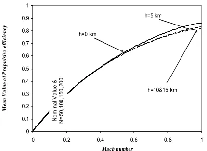
Figures 14 and 15 illustrate variance and mean of propulsive efficiency. As it can be seen in Figure 14, the values derived from N different points of uncertain parameters and nominal values match entirely. Also, Figure 15 depicts that propulsive efficiency is of insignificant range and may safely be considered as robust against uncertainties.

Figures 16 and 17 illustrate mean and variance of overall efficiency. Similar to what mentioned about Figure 12, the values of mean derived from N different point match each other and achieved curve exhibits an insignificant difference with that of nominal values. Further, as it can be seen in Figure 17, the variance of overall efficiency which reaches its maximum within the range of 0.6 to 0.7 Mach numbers is of an insignificant value. Therefore, based on the analysis of these two figures, overall efficiency may be safely assumed as robust against uncertainties.

The curves of mean and variance of performance functions are of crucial importance in robust and optimal design of turbofan engines. In robust optimization, if the purpose is to minimize (maximize) an objective function, the mean value is minimized (maximized) and the value of variance is minimized (minimized) [18].

Figure 8. Mean value of Thrust for N points of each uncertainty₍h_PR,h_b), considering nominal values of these parameters.

Figure9. Variance of Thrust for N points of each uncertain parameter(hPR,hb).

Figure10. Mean value of Thrust specific fuel consumption for N points of each uncertainty₍h_PR,h_b), considering nominal values of these parameters.

Figure11. Variance of Thrust specific fuel consumption for N points of each uncertain parameter₍h_PR,h_b).

0 50000 100000 150000 200000 250000 300000

0 0.2 0.4 0.6 0.8 1

Mach number

M

ea

n

V

al

ue

o

f T

hr

u

st

(N)

N

om

ina

l V

al

ue

&

N

=

50

,100,

1

50,200

h=0 km

h=5 km

h=10 km

h=15 km

-50 0 50 100 150 200 250 300 350 400 450

0 0.2 0.4 0.6 0.8 1

Mach number

V

ar

ia

nc

e

of T

hr

ust

(N)

h=

10 _km

N=50,100, 150,200

N=50,100 ,150,200

h=

5

km

h=

0

km

N=50,100, 150,200

h=

15 _km

N=50,100,150,200

9 11 13 15 17 19 21

0 0.2 0.4 0.6 0.8 1

Mach number

M

ea

n

V

al

ue

o

f

T

h

ru

st

s

p

ec

if

ic

f

u

el

c

o

ns

u

m

p

ti

o

n

[(

m

g/

se

c)

/N]

Nominal Value N=50,100 ,150,200

h=0 km h=5 km

h=10 km h=15 km

0 0.005 0.01 0.015 0.02 0.025 0.03 0.035 0.04 0.045 0.05

0 0.2 0.4 0.6 0.8 1

Mach number

V

ar

ia

nce

o

f T

hr

us

t s

pe

ci

fi

c

fu

el

c

on

su

m

pt

io

n

[(

m

g/

sec

)/

N]

N=200

N=150

N=100

Figure 12. Mean value of Thermal efficiency for N points of each uncertainty(hPR,hb), considering nominal values of these parameters.

Figure 15.Variance of Propulsive efficiency for N points of each uncertain parameter(hPR,hb).

Figure 13. Variance of Thermal efficiency for N points of each uncertain parameter(hPR,hb).

Figure 16. Mean value of Overall efficiency for N points of each uncertainty(h_PR,h_b), considering nominal values of these parameters.

Figure 14. Mean value of propulsive efficiency for N points of each uncertainty (hPR,hb) considering nominal values of these parameters.

Figure 17.Variance of Overall efficiency for N points of each uncertain parameter₍h_PR,h_b).

0.1 0.15 0.2 0.25 0.3 0.35 0.4 0.45

0 0.2 0.4 0.6 0.8 1

Mach number

M

ea

n

V

al

ue

o

f T

he

rm

al

e

ff

ic

ie

ncy

Nominal Value

N=50,100,150,200

Nominal V alue

N=50,100,150,200

0.00E+00 1.00E-09 2.00E-09 3.00E-09 4.00E-09 5.00E-09 6.00E-09 7.00E-09 8.00E-09 9.00E-09

0 0.2 0.4 0.6 0.8 1 Mach number

V

a

ri

an

ce

o

f

P

ro

p

ul

si

ve

e

ff

ic

ie

n

cy

N=100,150,200

N=50

0 0.000002 0.000004 0.000006 0.000008 0.00001 0.000012

0 0.2 0.4 0.6 0.8 1

Mach number

V

ar

ia

nc

e

of

T

he

rm

al

e

ff

ic

ie

ncy

N=50 N=100

N=150,200

0 0.05 0.1 0.15 0.2 0.25

0 0.2 0.4 0.6 0.8 1

Mach number

M

ea

n

va

lu

e

of

Ov

er

al

l e

ff

ic

ie

ncy

Nominal Value

N=50,100,150,200

0 0.1 0.2 0.3 0.4 0.5 0.6 0.7 0.8 0.9 1

0 0.2 0.4 0.6 0.8 1

Mach number

M

ea

n

V

alu

e

of

P

ro

pul

si

ve

e

ff

ic

ie

ncy

N

om

in

al

V

al

ue

&

N

=

50

,1

00

,1

50

,2

00

h=0 km

h=5 km

h=10&15 km

0.00E+00 5.00E-07 1.00E-06 1.50E-06 2.00E-06 2.50E-06 3.00E-06 3.50E-06

0 0.2 0.4 0.6 0.8 1

Mach number

V

ar

ia

nce

o

f O

ve

ra

ll

e

ff

ic

ie

ncy

N=50

N=100

8. CONCLUSION

In this paper, the impacts of uncertainties of burner efficiency as well as fuel heating value on performance functions of turbofan engine have been studied employing Monte Carlo sampling method, and the results have been drawn as curves based on inlet Mach number and various flight altitudes. It has been shown that the uncertainties do not exhibit significant impacts on thrust as well as thermal, propulsive and overall efficiencies and the mentioned functions are robust to the uncertainties. Further, the impacts of uncertainties on specific fuel consumption have been studied. This study can be of high importance for yielding a robust optimal design of turbofan engines.

9. REFERENCES

1. Kang, Z., “Robust design optimization of structure under uncertainties”, P.H.D Thesis, The university of Stuttgart, (2005).

2. Zhang, Z., “Design for uncertainties of sheet metal forming process”, PhD thesis, The Ohio state university, (2007).

3. Papadrakakis, M., Lagaros, N. D. and Plevris, V., “Structural Optimization Considering the Probabilistic System Response”,

Theoretical and Applied Mechanics, Vol. 31, (2004), 361-394.

4. Papadrakakis, M., Lagaros, N. D. and Plevris, V., “Design optimization of steel structures considering uncertainties”,

Engineering Structures, Vol. 27, (2005), 1408–1418.

5. Lagaros, N. D., Plevris, V. and Papadrakakis, M., “Reliability based robust design optimization of steel structures”,

International Journal for Simulation and Multidisciplinary Design Optimization, Vol. 1, (2007), 19-29.

6. Kumar, A., Nair, P. B., Keane, A. J. and Shahpar, Sh., “Robust design using Bayesian Monte Carlo”, International Journal for Numerical Methods in Engineering, Vol. 73, (2008), 1497– 1517.

7. Lalonde, N., “Multi objective Optimization Algorithm Benchmarking and Design Under Parameter Uncertainty”, Master Thesis, Queen's University, (2009).

8. Mattingly, J. D., “Elements of Gas Turbine Propultion”, AIAA Education series, Virginia,(2006).

9. Mattingly, J. D., Heiser, W. H. and Pratt, D. T., “Aircraft Engine Design”, 2nd _{ed. AIAA Education Series, Reston , (2002).}

10. Cohen, H., Rogers, G. and Saravanamuttoo, H., “Gas turbine theory”, 5th _{ed., Prentice Hall, New Jersey, (2001).}

11. Walsh, Ph. and Fletcher, P., “Gas Turbine Performance”, 2nd _ed.,

Wiley Blackwell, Derby, (2004).

12. Oates, G. C., “Aerothermodynamics of Gas Turbine and Rocket Propulsion”, 3rd _{ed., AIAA Education Series, Reston ,(1997).}

13. Gorji, M., Kazemi, A. and Ganji, D. D., “Thermodynamic Study of Turbofan Engine in Off-Design Conditions”, Journal of Basic and Applied Scientific Research, Vol. 2, (2012), 11239-11253.

14. Montegomery, D. C. and Runger, G. C., “Applied Statistics and Probability for Engineers”, 4th _{ed., Wiley, (2006).}

15. Shapiro, A. “Monte Carlo simulation approach to stochastic programming”, Proceedings of the Simulation Conference,

(2001), Vol. 1, 428-431.

16. Liu, J. S., “Monte Carlo Strategies in Scientific Computing”, 1st

ed., Springer, (2008).

17. Shaul, M., “Applications of Monte Carlo Method in Science and Engineering”, print ed., In Tech, (2011).

18. Smith, B. A., Kenny, S. and Crespo, L.G., “Probabilistic Parameter Uncertainty Analysis of Single Input Single Output Control Systems”, Langley Research Center, Virginia, (2005)

Uncertainties due to Fuel Heating

Value and Burner Efficiency on Performance

Functions of Turbofan Engines Using Monte Carlo Simulation

M. Gorji, A. Kazemi, D. D.Ganji

Department of Mechanical Engineering, Babol Noshirvani University of Technology, Babol, Iran

P A P E R I N F O

Paper history:

Received 26 May 2013

received in revised form 22 September 2013 Accepted 07 November 2013

Keywords: Monte Carlo Uncertainty Turbofan Engine

هﺪﯿﮑﭼ

ﯽﻣﯽﺳرﺮﺑﻦﻓﻮﺑرﻮﺗرﻮﺗﻮﻣيدﺮﮑﻠﻤﻋﻊﺑاﻮﺗيورﺮﺑقاﺮﺘﺣاقﺎﺗانﺎﻣﺪﻧاروﺖﺧﻮﺳﯽﺗراﺮﺣشزراﯽﻨﯿﻌﻣﺎﻧتاﺮﺛاﻪﻟﺎﻘﻣﻦﯾارد

دﻮﺷ

.

ﯽﻨﺤﻨﻣ

وﻦﯿﮕﻧﺎﯿﻣيﺎﻫ

نﺎﻣﺪﻧاروﺖﺧﻮﺳهﮋﯾوفﺮﺼﻣ،ﺶﻧارﻊﺑاﻮﺗياﺮﺑﺲﻧﺎﯾراو

ﺮﻈﻧردﺎﺑﯽﻠﮐوﯽﺗراﺮﺣ،ﺶﻧاريﺎﻫ

ﯽﻨﯿﻌﻣﺎﻧﻦﺘﻓﺮﮔ

زاوﺮﭘﺖﻋﺮﺳﺐﺴﺣﺮﺑهﺪﺷدﺎﯾيﺎﻫ

عﺎﻔﺗرارد

وﻢﺳريزاوﺮﭘﻒﻠﺘﺨﻣيﺎﻫ

درﻮﻣ

ﯽﻣراﺮﻗﻞﯿﻠﺤﺗ

دﺮﯿﮔ

.

ﯽﺳرﺮﺑﺎﺑ

ﯽﻣﯽﻨﯿﻌﻣﺎﻧتاﺮﺛا

ﺮﯾدﺎﻘﻣناﻮﺗ

ﻖﯿﻗدترﻮﺻﻪﺑارﺮﻈﻧدرﻮﻣفﺪﻫﻊﺑاﻮﺗ

ﺮﺗ ﺶﯿﭘ

دﻮﻤﻧﯽﻨﯿﺑ

.

وﻪﻨﯿﻬﺑﯽﺣاﺮﻃياﺮﺑﯽﺳرﺮﺑﻦﯾاﺞﯾﺎﺘﻧ

رﺎﯿﺴﺑﻦﻓﻮﺑرﻮﺗيﺎﻫرﻮﺗﻮﻣموﺎﻘﻣ

ﯽﻣيروﺮﺿ

ﺪﺷﺎﺑ

.

ﺮﺛاﯽﺳرﺮﺑ

ﯽﻨﯿﻌﻣﺎﻧﻦﯾا

ﻪﯿﺒﺷشورﻂﺳﻮﺗﻦﻓﻮﺑرﻮﺗرﻮﺗﻮﻣردﺎﻫ

ﺖﻧﻮﻣيزﺎﺳ

شورزاﻪﮐﺖﻓﺮﮔﺪﻫاﻮﺧترﻮﺻﻮﻟرﺎﮐ

ﺖﺳاﯽﺗﻻﺎﻤﺘﺣاﻞﯿﻠﺤﺗيﺎﻫ

.

doi: 10.5829/idosi.ije.2014.27.07a.16